A Simple Model

Section 14.1 A Simple Model

In this section we are going to model the motion of an object attached to the free end of a spring which has its other end fixed as shown in Figure 14.1.1. To construct this model set up an axis with its origin at the centre of the object when the object-spring system is in equilibrium and with the positive direction going upward. With respect to this axis assume that without the object attached the end of the spring is at \(y=N\text{.}\) Now, imagine that the object is pulled down \(L\) units (with respect to the axis) and then let go.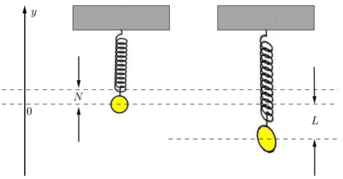

Our models for the motion of the object will be based Hooke's Law and Newton's second law of motion.

Definition 14.1.2. Hooke's Law.

If a spring is stretched (compressed) \(U\) units beyond its natural position then it pulls (pushes) with a force, \(\mathbf{F_r}\text{,}\) of magnitude

\begin{equation*} \vert \mathbf{F_r} \vert =kU, \hspace{5mm} k>0 \end{equation*}

where the value of \(k\) depends on the properties of the spring itself.

Common terminology is to call the force \(\mathbf{F_r}\) the restoring force and the constant \(k\) the spring constant.

Definition 14.1.3. Newton's Second Law of Motion.

The acceleration, \(\mathbf{a}\text{,}\) of an object as produced by a net force, \(\mathbf{F}\text{,}\) is directly proportional to the magnitude of the net force, in the same direction as the net force, and inversely proportional to the mass, \(m\text{,}\) of the object, i.e. \(\mathbf{F}=m\mathbf{a}\text{.}\)

So, now consider the forces acting on the object at any time \(t\) after the object has been pulled down and released. In our initial model we will assume that there are just two forces acting on the object as shown in Figure 14.1.4: firstly the force due to gravity, \(\mathbf{F_g}\text{,}\) and secondly the restoring force, \(\mathbf{F_r}\text{,}\) due to the spring.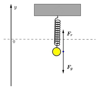

With the axis as set up in Figure 14.1.4 (or Figure 14.1.1), \(\mathbf{F_g}\) will always act in the negative direction. However, \(\mathbf{F_r}\) will be positive when the displacement of the object is less than \(N\) and negative when the displacement of the object is greater than \(N\) (i.e. the restoring force always acts in the direction of the natural position of the spring). Notice that since the motion of the object is one dimensional we can represent the relevant vector quantities by real numbers. The sign of the number will give us the direction of the vector.

Thus, the force due to gravity is constant and is given by

\begin{equation*} F_g=-mg \end{equation*}

where \(m\) is the mass of the object and \(g\) is the acceleration due to gravity. (This follows from Newton's Universal Law of Gravitation and Newton's second law of motion.). If \(y\) represents the displacement of (the centre of) the object then from Hooke's Law

\begin{equation*} F_r=-k(y-N) \end{equation*}

where \(k\gt 0\) is the spring constant. Notice that the negative sign is needed in this relationship to make the restoring force act in the correct direction. Thus the net force acting on the object is

\begin{equation*} F=F_g+F_r=-mg-ky+kN \end{equation*}

Now if we let \(a\) be the acceleration of the object, then from Newton’s second law of motion

\begin{align*} ma \amp=F\\ m\frac{d^2y}{dt^2} \amp=-mg-ky+kN \end{align*}

Thus we are able to model the displacement of the object via a 2nd order linear DE with constant coefficients, along with the initial conditions

\begin{equation*} y(0)=-L,\hspace{5mm} y'(0)=0 \end{equation*}

We can further simplify the DE by noting that when the object-spring system is in equilibrium the net force is zero and hence

\begin{equation*} -mg+kN=0 \end{equation*}

Using this, the model simplifies to

\begin{equation} \frac{d^2y}{dt^2}+\left(\frac{k}{m}\right)y=0, \hspace{5mm}y(0)=-L, \hspace{5mm}y'(0)=0,\hspace{5mm} k>0,\hspace{5mm} m>0\label{Equation_14_1_1}\tag{14.1.1} \end{equation}

which is an initial-value problem involving a homogeneous 2nd order linear DE with constant coefficients.

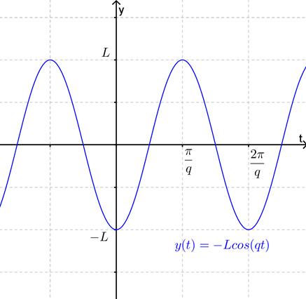
Using the methods outlined in Chapter 12 we find that the general solution to (14.1.1) is

\begin{equation*} y(t)=C_1\cos(qt)+C_2\sin(qt) \end{equation*}

where \(q=\sqrt{\frac{k}{m}}\) is called the natural frequency of the system. (Note that \(q\) should probably be called the "natural angular frequency" since the frequency of \(y\) is \(\frac{q}{2\pi}\text{.}\)) The derivative of \(y\) is

\begin{equation*} y'(t)=-C_1\sin(qt)+C_2\cos(qt) \end{equation*}

and hence from the initial conditions we find that \(C_1=-L\) and \(C_2=0\text{.}\) Thus the solution to the initial-value problem is

\begin{equation*} y(t)=-L\cos(qt) \end{equation*}

As shown in Figure 14.1.5, this solution is telling us that (under the assumptions of the model) the motion of the object will be periodic about the equilibrium position i.e. will be simple harmonic motion.

Of course real springs do not oscillate forever and so we conclude that our model must have ignored some important details (e.g. air resistance, frictional forces etc.) Despite this obvious shortcoming we will use this simple model as the basis for looking at more complicated contexts.