Section 14.3 Adding an External Force
In our final model we will look at the situation where some other external force, \(\mathbf{F_e}\text{,}\) is also acting on the object along the \(y\)-axis, as shown in Figure 14.3.1. This context has many applications, especially in engineering, although in most applications the context doesn't actually look like the diagram shown in Figure 14.3.1. For example if the top of a power pole is pulled to one side and let go it will behave like an object-spring system with damping. Now when a wind blows past the pole it is possible that aerodynamic effects can result in an oscillating side force acting on the pole. 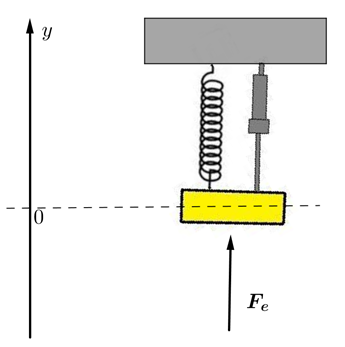
Then the net force acting on the object will be
and hence the motion of the object can be modelled by the DE
Following the same steps as in the previous section we can, therefore, write our model as
So now the DE is a non-homogeneous 2nd order linear DE with constant coefficients. The general solution is constructed from the complementary solution and a particular solution. We know the complementary solution from our previous model. From that model we know that the complementary solution always tends to \(0\) as \(t\rightarrow\infty\text{.}\) Thus the long term behaviour of this system is determined by the particular solution to (14.3.1). From Chapter 13 we know that a particular solution will be of the form
Substituting into Chapter 13 and equating coefficients gives
Since it is easier to interpret we will write \(y_p(t)\) as a single trigonometric function. Thus let
Using some standard trigonometric identities it can be shown that
Thus
From this we can conclude that the long term response of our damped object-spring system to forcing by an external force \(F_e(t)=A\cos(\alpha t)\) is to oscillate at the forcing angular frequency, \(\alpha\text{,}\) and with an amplitude
that is the amplitude of the external force multiplied by the factor
Notice that, since for a given object-spring system \(p\) and \(q\) are fixed values, this factor \(M\) is a function of the forcing angular frequency \(\alpha\text{.}\) Figure 14.3.2 shows graphs of \(M(\alpha)\) for various values of \(p\) (which relates to the damping coefficient) when \(q\) (which relates to the stiffness coefficient) is held constant at \(q=1\text{.}\) In fact, it can be shown that if the damping parameter \(\delta\) (\(=\frac{p}{q}\)) is small then \(M\) has a maximum when the forcing frequency is near the natural frequency of the system and further that this maximum tends to infinity as \(\delta\rightarrow 0\text{.}\) 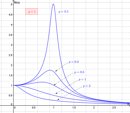
The significance of this analysis is the insight that if our damped object-spring system is subjected to an external oscillatory force near the natural frequency of the system it will respond with large amplitude motion unless the system is sufficiently damped. This phenomenon is known as resonance.
Exercises Example Tasks
1.
Determine the values of \(a\) and \(b\) in the DE \(\frac{d^2x}{dt^2}+2a\frac{dx}{dt}+bx=0\) that give the damped object-spring system a damping parameter of \(0.5\) and a natural frequency of \(2\text{.}\)
2.
A beam that is fixed rigidly at one end and designed to support a load at the other end is called a cantilever. If the cantilever is designed only to deflect a "small" amount under its load then it is reasonable to assume that the size of the deflection of the tip of the cantilever is proportional to the load applied. When such a cantilever is deflected beyond (or less than) its equilibrium position the cantilever exerts a restoring force toward the equilibrium position. So long as the deflection is reasonably small and the mass of the object is large compared to the mass of the cantilever this restoring force is proportional to the deflection. Show that the resulting motion of the tip of the cantilever can be modelled under these assumptions via a homogeneous 2nd order linear DE. 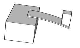
3.
Show that if \(a\cos(\alpha t)+b\sin(\alpha t)=C\cos(\alpha t-\beta)\) then