Section 19.2 Finding Eigenvalues and Eigenvectors
For the square matrix \(A\text{,}\) the eigenvalues and associated eigenvectors are defined by the equation
\begin{equation}
A\mathbf{x}=\lambda\mathbf{x}\label{Eq-Eigenvector_definition}\tag{19.2.1}
\end{equation}
Thus, we want to find values of \(\lambda\text{,}\) and associated vectors \(\mathbf{x}\text{,}\) that satisfy this equation. To do this, rearrange (19.2.1) to obtain
\begin{equation*}
A\mathbf{x}-\lambda\mathbf{x}=\mathbf{0}
\end{equation*}
which can be written as
\begin{equation*}
A\mathbf{x}-\lambda I\mathbf{x}=\mathbf{0}
\end{equation*}
or
\begin{equation}
(A-\lambda I)\mathbf{x}=\mathbf{0}\label{Eq-Eigenvector_definition_with_identity_matrix}\tag{19.2.2}
\end{equation}
where \(I\) is the identity matrix of order \(n\text{.}\) Since (19.2.2) is a homogeneous system of linear equations it will only have a non-zero solution when
\begin{equation}
\det(A-\lambda I)=0\label{Eq-Eigenvector_definition_with_determinant}\tag{19.2.3}
\end{equation}
Definition 19.2.1 .
The eigenvalues, \(\lambda\text{,}\) of the \(n\times n\) matrix \(A\) are found by solving the characteristic equation
\begin{equation*}
\det(A-\lambda I)=0
\end{equation*}
The eigenvectors of the matrix \(A\) are found by solving the homogeneous linear system of equations
\begin{equation*}
(A-\lambda I)\mathbf{x}=\mathbf{0}
\end{equation*}
for each eigenvalue \(\lambda\text{.}\)
Example 19.2.2 .
Find all eigenvalues and associated eigenvectors for
\begin{equation*}
A=\begin{pmatrix} 2 \amp 1 \\ 1 \amp 2 \end{pmatrix}
\end{equation*}
Answer .
For \(\lambda=1\text{,}\) the eigenvectors take the form \(\mathbf{x}=t\begin{pmatrix} -1 \\ 1 \end{pmatrix}\text{.}\)
For \(\lambda=3\text{,}\) the eigenvectors take the form \(\mathbf{x}=t\begin{pmatrix} 1 \\ 1 \end{pmatrix}\text{.}\)
Solution .
The eigenvalues, \(\lambda\text{,}\) of \(A\) satisfy the characteristic equation
\begin{equation*}
\det(A-\lambda I)=0
\end{equation*}
Since
\begin{equation*}
A-\lambda I=\begin{pmatrix} 2\amp 1 \\ 1\amp 2 \end{pmatrix}-\lambda \begin{pmatrix} 1\amp 0 \\ 0\amp 1 \end{pmatrix}=\begin{pmatrix} 2-\lambda \amp 1 \\ 1\amp 2-\lambda \end{pmatrix}
\end{equation*}
the characteristic equation is
\begin{align*}
\det\begin{pmatrix} 2-\lambda \amp 1 \\ 1\amp 2-\lambda \end{pmatrix} \amp =0\\
(2-\lambda)^2-1 \amp =0\\
\lambda^2-4\lambda+3 \amp =0
\end{align*}
Thus the eigenvalues for \(A\) are
\begin{equation*}
\lambda=1 \textrm{ and } \lambda=3
\end{equation*}
To find the eigenvectors associated with each of these eigenvalues we follow the procedure illustrated in Example 19.1.5 , i.e. solve the homogeneous system of linear equations
\begin{equation*}
(A-\lambda I)\mathbf{x}=\mathbf{0}
\end{equation*}
for each eigenvalue.
When \(\lambda=1\) the augmented matrix and its reduced row echelon form are
\begin{equation*}
\begin{pmatrix} 1 \amp 1 \amp 0 \\ 1 \amp 1 \amp 0 \end{pmatrix} \sim \begin{pmatrix} 1 \amp 1 \amp 0 \\ 0 \amp 0 \amp 0 \end{pmatrix} \begin{matrix} \\ \hspace{5mm} R_2'=R_2-R_1 \end{matrix}
\end{equation*}
Thus, the eigenvectors take the form
\begin{align*}
\mathbf{x} \amp =\begin{pmatrix}x_1 \\ x_2\end{pmatrix} \textrm{ where } x_1+x_2=0\\
\Rightarrow \mathbf{x} \amp =\begin{pmatrix} -t \\ t \end{pmatrix}=t\begin{pmatrix} -1 \\ 1 \end{pmatrix}
\end{align*}
When \(\lambda=3\) the augmented matrix and its reduced row echelon form are
\begin{equation*}
\begin{pmatrix} -1 \amp 1 \amp 0 \\ 1 \amp -1 \amp 0 \end{pmatrix} \sim \begin{pmatrix} -1 \amp 1 \amp 0 \\ 0 \amp 0 \amp 0 \end{pmatrix} \begin{matrix} \\ \hspace{5mm} R_2'=R_2+R_1 \end{matrix}
\end{equation*}
Thus, the eigenvectors take the form
\begin{align*}
\mathbf{x} \amp =\begin{pmatrix}x_1 \\ x_2\end{pmatrix} \textrm{ where } -x_1+x_2=0\\
\Rightarrow \mathbf{x} \amp =\begin{pmatrix} t \\ t \end{pmatrix}=t\begin{pmatrix} 1 \\ 1 \end{pmatrix}
\end{align*}
As always, you can very easily check that these vectors are indeed eigenvectors by performing the matrix multiplication \(A\mathbf{x}\text{.}\)
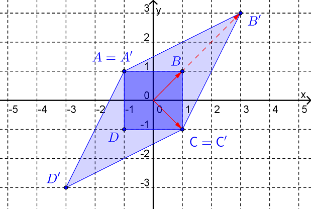
As an aside, we can get some geometric insight if we consider \(A\) as the matrix of a plane transformation, (even though \(A\) isn’t the matrix for any well known transformation). Figure 19.2.3 shows the result of applying \(A\) to a square centred on the origin.
Figure 19.2.3. Informally, the effect of \(A\) is to pull the square out along the diagonal joining vertices \(B\) and \(D\text{.}\) Thus vectors along this diagonal will be mapped to scalar multiples of themselves while vectors along the diagonal joining vertices \(A\) and \(C\) will be left unchanged.
Example 19.2.4 .
Find all eigenvalues and associated eigenvectors for
\begin{equation*}
A=\begin{pmatrix} 1 \amp 2 \\ 3 \amp 4 \end{pmatrix}
\end{equation*}
Answer .
For \(\lambda=\dfrac{5+\sqrt{33}}{2}\text{,}\) the eigenvectors take the form \(\mathbf{x}=t\begin{pmatrix} 4 \\ 3+\sqrt{33} \end{pmatrix}\text{.}\)
For \(\lambda=\dfrac{5-\sqrt{33}}{2}\text{,}\) the eigenvectors take the form \(\mathbf{x}=t\begin{pmatrix} 4 \\ 3-\sqrt{33} \end{pmatrix}\text{.}\)
Solution .
The characteristic equation for \(A\) is
\begin{align*}
\det\begin{pmatrix} 1-\lambda \amp 2 \\ 3\amp 4-\lambda \end{pmatrix} \amp =0\\
(1-\lambda)(4-\lambda)-6 \amp =0\\
\lambda^2-5\lambda-2 \amp =0
\end{align*}
Thus the eigenvalues for \(A\) are
\begin{equation*}
\lambda=\frac{5\pm\sqrt{33}}{2}\approx 5.37, -0.37
\end{equation*}
Clearly the eigenvalues don't always turn out to be nice numbers, even when the matrix is quite simple. The eigenvectors will also turn out to be rather complicated.
When \(\lambda=\dfrac{5+\sqrt{33}}{2}\) the augmented matrix and its reduced row echelon form are
\begin{equation*}
\begin{pmatrix} 1-\left(\frac{5+\sqrt{33}}{2} \right) \amp 2 \amp 0 \\ 3 \amp 4-\left(\frac{5+\sqrt{33}}{2} \right) \amp 0 \end{pmatrix} \sim \begin{pmatrix} \frac{-3-\sqrt{33}}{2} \amp 2 \amp 0 \\ 0 \amp 0 \amp 0 \end{pmatrix}
\end{equation*}
Thus, the eigenvectors take the form
\begin{align*}
\mathbf{x} \amp =\begin{pmatrix} x_1 \\ x_2 \end{pmatrix} \textrm{ where } \left(\frac{-3-\sqrt{33}}{2}\right)x_1+2x_2=0 \\
\Rightarrow \mathbf{x} \amp =\begin{pmatrix} 4t \\ t(3+\sqrt{33}) \end{pmatrix} = t\begin{pmatrix} 4 \\ 3+\sqrt{33} \end{pmatrix}
\end{align*}
When \(\lambda=\dfrac{5-\sqrt{33}}{2}\) the augmented matrix and its reduced row echelon form are
\begin{equation*}
\begin{pmatrix} 1-\left(\frac{5-\sqrt{33}}{2} \right) \amp 2 \amp 0 \\ 3 \amp 4-\left(\frac{5-\sqrt{33}}{2} \right) \amp 0 \end{pmatrix} \sim \begin{pmatrix} \frac{-3+\sqrt{33}}{2} \amp 2 \amp 0 \\ 0 \amp 0 \amp 0 \end{pmatrix}
\end{equation*}
Thus, the eigenvectors take the form
\begin{align*}
\mathbf{x} \amp =\begin{pmatrix} x_1 \\ x_2 \end{pmatrix} \textrm{ where } \left(\frac{-3+\sqrt{33}}{2}\right)x_1+2x_2=0 \\
\Rightarrow \mathbf{x} \amp =\begin{pmatrix} 4t \\ t(3-\sqrt{33}) \end{pmatrix} = t\begin{pmatrix} 4 \\ 3-\sqrt{33} \end{pmatrix}
\end{align*}
Example 19.2.5 .
Find all eigenvalues and associated eigenvectors for
\begin{equation*}
A=\begin{pmatrix} 1 \amp 2 \\ 2 \amp 4 \end{pmatrix}
\end{equation*}
Answer .
For \(\lambda=0\text{,}\) the eigenvectors take the form \(\mathbf{x}=t\begin{pmatrix} -2 \\ 1 \end{pmatrix}\text{.}\)
For \(\lambda=5\text{,}\) the eigenvectors take the form \(\mathbf{x}=t\begin{pmatrix} 1 \\ 2 \end{pmatrix}\text{.}\)
Solution .
The characteristic equation for \(A\) is
\begin{align*}
\det\begin{pmatrix} 1-\lambda \amp 2 \\ 2\amp 4-\lambda \end{pmatrix} \amp =0\\
(1-\lambda)(4-\lambda)-4 \amp =0\\
\lambda^2-5\lambda \amp =0
\end{align*}
Thus the eigenvalues for \(A\) are
\begin{equation*}
\lambda=0, 5
\end{equation*}
When \(\lambda=0\) the augmented matrix and its reduced row echelon form are
\begin{equation*}
\begin{pmatrix} 1 \amp 2 \amp 0 \\ 2 \amp 4 \amp 0 \end{pmatrix} \sim \begin{pmatrix} 1 \amp 2 \amp 0 \\ 0 \amp 0 \amp 0 \end{pmatrix}
\end{equation*}
Thus, the eigenvectors take the form
\begin{align*}
\mathbf{x} \amp =\begin{pmatrix} x_1 \\ x_2 \end{pmatrix} \textrm{ where } x_1+2x_2=0 \\
\Rightarrow \mathbf{x} \amp =\begin{pmatrix} -2t \\ t \end{pmatrix} = t\begin{pmatrix} -2 \\ 1 \end{pmatrix}
\end{align*}
When \(\lambda=5\) the augmented matrix and its reduced row echelon form are
\begin{equation*}
\begin{pmatrix} -4 \amp 2 \amp 0 \\ 2 \amp -1 \amp 0 \end{pmatrix} \sim \begin{pmatrix} 2 \amp -1 \amp 0 \\ 0 \amp 0 \amp 0 \end{pmatrix}
\end{equation*}
Thus, the eigenvectors take the form
\begin{align*}
\mathbf{x} \amp =\begin{pmatrix} x_1 \\ x_2 \end{pmatrix} \textrm{ where } 2x_1-x_2=0 \\
\Rightarrow \mathbf{x} \amp =\begin{pmatrix} t \\ 2t \end{pmatrix} = t\begin{pmatrix} 1 \\ 2 \end{pmatrix}
\end{align*}
Notice that when \(0\) is an eigenvalue of \(A\) the system of equations that are solved to find the associated eigenvectors, i.e.
\begin{equation*}
(A-\lambda I)\mathbf{x}=\mathbf{0}
\end{equation*}
reduces to
\begin{equation*}
A\mathbf{x}=\mathbf{0}
\end{equation*}
Since \(0\) is an eigenvalue of \(A\) we know that this system must have non-zero solutions which in turn tells us that \(A\) is not invertible. Thus, if \(A\) has \(0\) as an eigenvalue it will not be invertible and vice versa.
Example 19.2.6 .
Find all eigenvalues and associated eigenvectors for
\begin{equation*}
A=\begin{pmatrix} 0 \amp 1 \\ -1 \amp 0 \end{pmatrix}
\end{equation*}
Answer .
For \(\lambda=i\text{,}\) the eigenvectors take the form \(\mathbf{x}=t\begin{pmatrix} 1 \\ i \end{pmatrix}\text{.}\)
For \(\lambda=-i\text{,}\) the eigenvectors take the form \(\mathbf{x}=t\begin{pmatrix} -1 \\ i \end{pmatrix}\text{.}\)
Solution .
The characteristic equation for \(A\) is
\begin{align*}
\det\begin{pmatrix} 0-\lambda \amp 1 \\ -1 \amp 0-\lambda \end{pmatrix} \amp =0 \\
\lambda^2+1 \amp =0
\end{align*}
This equation has no real solutions and so \(A\) does not have any real eigenvalues. (Notice that \(A\) is the matrix for a rotation in the plane about the origin and through \(-\frac{\pi}{2}^c\text{.}\) ) However there are applications where it is advantageous to allow the eigenvalues and eigenvectors to be complex. So, proceeding as before, the eigenvalues for \(A\) are
\begin{equation*}
\lambda=\pm i
\end{equation*}
When \(\lambda=i\) the augmented matrix and its reduced row echelon form are
\begin{equation*}
\begin{pmatrix} -i \amp 1 \amp 0 \\ -1 \amp -i \amp 0 \end{pmatrix} \sim \begin{pmatrix} 1 \amp i \amp 0 \\ 0 \amp 0 \amp 0 \end{pmatrix}
\end{equation*}
Thus, the eigenvectors take the form
\begin{align*}
\mathbf{x} \amp =\begin{pmatrix} x_1 \\ x_2 \end{pmatrix} \textrm{ where } x_1+ix_2=0 \\
\Rightarrow \mathbf{x} \amp =\begin{pmatrix} t \\ ti \end{pmatrix} = t\begin{pmatrix} 1 \\ i \end{pmatrix}
\end{align*}
When \(\lambda=-i\) the augmented matrix and its reduced row echelon form are
\begin{equation*}
\begin{pmatrix} i \amp 1 \amp 0 \\ -1 \amp i \amp 0 \end{pmatrix} \sim \begin{pmatrix} 1 \amp -i \amp 0 \\ 0 \amp 0 \amp 0 \end{pmatrix}
\end{equation*}
Thus, the eigenvectors take the form
\begin{align*}
\mathbf{x} \amp =\begin{pmatrix} x_1 \\ x_2 \end{pmatrix} \textrm{ where } x_1-ix_2=0 \\
\Rightarrow \mathbf{x} \amp =\begin{pmatrix} -t \\ ti \end{pmatrix} = t\begin{pmatrix} -1 \\ i \end{pmatrix}
\end{align*}
As we have seen the characteristic equation for a \(2\times 2\) matrix is always a polynomial of degree \(2\text{.}\) Once we allow complex solutions we can that every \(2\times 2\) matrix will have exactly \(2\) eigenvalues (so long as we count repeated roots). In fact, it can be shown that this result holds more generally. Every square matrix of order \(n\) has \(n\) eigenvalues (counting repeated roots).
Example 19.2.7 .
Find all eigenvalues and associated eigenvectors for
\begin{equation*}
A=\begin{pmatrix} 7 \amp 1 \amp -2 \\ -3 \amp 3 \amp 6 \\ 2 \amp 2\amp 2 \end{pmatrix}
\end{equation*}
Answer .
For \(\lambda=0\text{,}\) the eigenvectors take the form \(\mathbf{x}=t\begin{pmatrix} 1 \\ -3 \\ 2 \end{pmatrix}\text{.}\)
For \(\lambda=6\text{,}\) the eigenvectors take the form \(\mathbf{x}=s\begin{pmatrix} -1 \\ 1 \\ 0 \end{pmatrix}+t\begin{pmatrix} 2 \\ 0 \\ 1 \end{pmatrix}\text{.}\)
Solution .
The characteristic equation for \(A\) is
\begin{equation*}
\det\begin{pmatrix} 7-\lambda \amp 1 \amp -2 \\ -3 \amp 3-\lambda \amp 6 \\ 2 \amp 2\amp 2-\lambda \end{pmatrix}=0
\end{equation*}
Now, using the minors method and expanding along row 1,
\begin{align*}
\det\begin{pmatrix} 7-\lambda \amp 1 \amp -2 \\ -3 \amp 3-\lambda \amp 6 \\ 2 \amp 2\amp 2-\lambda \end{pmatrix} \amp =(7-\lambda)\begin{vmatrix} 3-\lambda \amp 6 \\ 2 \amp 2-\lambda \end{vmatrix}-1\begin{vmatrix} -3 \amp 6 \\ 2 \amp 2-\lambda \end{vmatrix}+(-2)\begin{vmatrix} -3 \amp 3-\lambda \\ 2 \amp 2 \end{vmatrix} \\
\amp = (7-\lambda)\{(3-\lambda)(2-\lambda)-12\}\\
\amp \quad \quad \quad \quad -\{(-3)(2-\lambda)-12\}-2\{-6-2(3-\lambda)\}\\
\amp = -\lambda^3+12\lambda^2-36\lambda
\end{align*}
Thus the eigenvalues for \(A\) satisfy
\begin{align*}
\lambda^3-12\lambda^2+36\lambda \amp =0\\
\lambda(\lambda-6)^2 \amp =0\\
\lambda \amp = 0, 6
\end{align*}
Since \(\lambda=6\) is a repeated root of the characteristic equation we say that this is an eigenvalue of multiplicity \(2\text{.}\) Also, since \(\lambda=0\) is an eigenvalue of \(A\) we know that \(A\) is not invertible.
When \(\lambda=0\) the augmented matrix and its reduced row echelon form are
\begin{equation*}
\begin{pmatrix} 7 \amp 1 \amp -2 \amp 0 \\ -3 \amp 3 \amp 6 \amp 0 \\ 2 \amp 2 \amp 2 \amp 0 \end{pmatrix} \sim \begin{pmatrix} 1 \amp 0 \amp -\frac{1}{2} \amp 0 \\ 0 \amp 1 \amp \frac{3}{2} \amp 0 \\ 0 \amp 0 \amp 0 \amp 0 \end{pmatrix}
\end{equation*}
Thus, the eigenvectors take the form
\begin{align*}
\mathbf{x} \amp =\begin{pmatrix} x_1 \\ x_2 \\ x_3 \end{pmatrix} \textrm{ where } \begin{matrix} \hspace{3.5mm} x_1-x_3/2=0 \\ \hspace{2mm} x_2+3x_3/2=0 \end{matrix} \\
\Rightarrow \mathbf{x} \amp =\begin{pmatrix} t \\ -3t \\ 2t \end{pmatrix} = t\begin{pmatrix} 1 \\ -3 \\ 2 \end{pmatrix}
\end{align*}
When \(\lambda=6\) the augmented matrix and its reduced row echelon form are
\begin{equation*}
\begin{pmatrix} 1 \amp 1 \amp -2 \amp 0 \\ -3 \amp -3 \amp 6 \amp 0 \\ 2 \amp 2 \amp -4 \amp 0 \end{pmatrix} \sim \begin{pmatrix} 1 \amp 1 \amp -2 \amp 0 \\ 0 \amp 0 \amp 0 \amp 0 \\ 0 \amp 0 \amp 0 \amp 0 \end{pmatrix}
\end{equation*}
Thus, the eigenvectors take the form
\begin{align*}
\mathbf{x} \amp =\begin{pmatrix} x_1 \\ x_2 \\ x_3 \end{pmatrix} \textrm{ where } x_1+x_2-2x_3=0 \\
\Rightarrow \mathbf{x} \amp =\begin{pmatrix} -s+2t \\ s \\ t \end{pmatrix} = s\begin{pmatrix} -1 \\ 1 \\ 0 \end{pmatrix}+t\begin{pmatrix} 2 \\ 0 \\ 1 \end{pmatrix}
\end{align*}
Example 19.2.8 .
Find all eigenvalues and associated eigenvectors for
\begin{equation*}
A=\begin{pmatrix} 7 \amp 1 \amp -2 \\ 0 \amp 3 \amp 6 \\ 0 \amp 0 \amp 2 \end{pmatrix}
\end{equation*}
Answer .
For \(\lambda=2\text{,}\) the eigenvectors take the form \(\mathbf{x}=t\begin{pmatrix} 8 \\ -30 \\ 5 \end{pmatrix}\text{.}\)
For \(\lambda=3\text{,}\) the eigenvectors take the form \(\mathbf{x}=t\begin{pmatrix} -1 \\ 4 \\ 0 \end{pmatrix}\text{.}\)
For \(\lambda=7\text{,}\) the eigenvectors take the form \(\mathbf{x}=t\begin{pmatrix} 1 \\ 0 \\ 0 \end{pmatrix}\text{.}\)
Solution .
The characteristic equation for \(A\) is
\begin{equation*}
\det\begin{pmatrix} 7-\lambda \amp 1 \amp -2 \\ 0 \amp 3-\lambda \amp 6 \\ 0 \amp 0 \amp 2-\lambda \end{pmatrix}=0
\end{equation*}
Now, using the minors method and expanding down column 1,
\begin{align*}
\det\begin{pmatrix} 7-\lambda \amp 1 \amp -2 \\ 0 \amp 3-\lambda \amp 6 \\ 0 \amp 0\amp 2-\lambda \end{pmatrix} \amp =(7-\lambda)\begin{vmatrix} 3-\lambda \amp 6 \\ 0 \amp 2-\lambda \end{vmatrix}-0\begin{vmatrix} 1 \amp -2 \\ 0 \amp 2-\lambda \end{vmatrix}+0\begin{vmatrix} 1 \amp -2 \\ 3-\lambda \amp 6 \end{vmatrix} \\
\amp = (7-\lambda)\{(3-\lambda)(2-\lambda)-0\}-0+0\\
\amp = (7-\lambda)(3-\lambda)(2-\lambda)
\end{align*}
Thus the eigenvalues for \(A\) satisfy
\begin{equation*}
\lambda=2,3,7
\end{equation*}
When \(\lambda=2\) the augmented matrix and its reduced row echelon form are
\begin{equation*}
\begin{pmatrix} 5 \amp 1 \amp -2 \amp 0 \\ 0 \amp 1 \amp 6 \amp 0 \\ 0 \amp 0 \amp 0 \amp 0 \end{pmatrix} \sim \begin{pmatrix} 5 \amp 0 \amp -8 \amp 0 \\ 0 \amp 1 \amp 6 \amp 0 \\ 0 \amp 0 \amp 0 \amp 0 \end{pmatrix}
\end{equation*}
Thus, the eigenvectors take the form
\begin{align*}
\mathbf{x} \amp =\begin{pmatrix} x_1 \\ x_2 \\ x_3 \end{pmatrix} \textrm{ where } \begin{matrix} \hspace{2mm} 5x_1-8x_3=0 \\ \hspace{4mm} x_2+6x_3=0 \end{matrix} \\
\Rightarrow \mathbf{x} \amp =\begin{pmatrix} 8t \\ -30t \\ 5t \end{pmatrix} = t\begin{pmatrix} 8 \\ -30 \\ 5 \end{pmatrix}
\end{align*}
When \(\lambda=3\) the augmented matrix and its reduced row echelon form are
\begin{equation*}
\begin{pmatrix} 4 \amp 1 \amp -2 \amp 0 \\ 0 \amp 0 \amp 6 \amp 0 \\ 0 \amp 0 \amp -1 \amp 0 \end{pmatrix} \sim \begin{pmatrix} 4 \amp 1 \amp 0 \amp 0 \\ 0 \amp 0 \amp 1 \amp 0 \\ 0 \amp 0 \amp 0 \amp 0 \end{pmatrix}
\end{equation*}
Thus, the eigenvectors take the form
\begin{align*}
\mathbf{x} \amp =\begin{pmatrix} x_1 \\ x_2 \\ x_3 \end{pmatrix} \textrm{ where } \begin{matrix} \hspace{2mm} 4x_1+x_2=0 \\ \hspace{14.5mm} x_3=0 \end{matrix} \\
\Rightarrow \mathbf{x} \amp =\begin{pmatrix} -t \\ 4t \\ 0 \end{pmatrix} = t\begin{pmatrix} -1 \\ 4 \\ 0 \end{pmatrix}
\end{align*}
When \(\lambda=7\) the augmented matrix and its reduced row echelon form are
\begin{equation*}
\begin{pmatrix} 0 \amp 1 \amp -2 \amp 0 \\ 0 \amp -4 \amp 6 \amp 0 \\ 0 \amp 0 \amp -5 \amp 0 \end{pmatrix} \sim \begin{pmatrix} 0 \amp 1 \amp 0 \amp 0 \\ 0 \amp 0 \amp 1 \amp 0 \\ 0 \amp 0 \amp 0 \amp 0 \end{pmatrix}
\end{equation*}
Thus, the eigenvectors take the form
\begin{align*}
\mathbf{x} \amp =\begin{pmatrix} x_1 \\ x_2 \\ x_3 \end{pmatrix} \textrm{ where } \begin{matrix} \hspace{2mm} x_2=0 \\ \hspace{2mm} x_3=0 \end{matrix} \\
\Rightarrow \mathbf{x} \amp =\begin{pmatrix} t \\ 0 \\ 0 \end{pmatrix} = t\begin{pmatrix} 1 \\ 0 \\ 0 \end{pmatrix}
\end{align*}
As illustrated in Example 19.2.8 , for an upper triangular matrix the eigenvalues are the entries on the main diagonal. Unfortunately, we cannot use row reduction to find eigenvalues because equivalent matrices do not necessarily have the same eigenvalues. Interestingly though, it can be shown that sum of the eigenvalues of any square matrix is equal to the sum of the entries on the main diagonal (i.e. to the trace of the matrix).
To close this section, we can once again add one more statement to our theorem connecting the ideas that we have studied so far.
Theorem 19.2.9 .
Consider the non-homogenous system of \(n\) linear equations in \(n\) variables
\begin{equation*}
A\mathbf{x}=\mathbf{b}, \hspace{5mm} \mathbf{b\neq 0}
\end{equation*}
The following statements are equivalent:
The system has a unique solution.
\(A\mathbf{x}=\mathbf{0}\) has only the trivial solution \(\mathbf{x}=\mathbf{0}\)
The columns of \(A\) are linearly independent
\(A\) is invertible
\(\displaystyle det(A)\neq 0\)
\(0\) is not an eigenvalue of \(A\)
Exercises Example Tasks
1. Find all eigenvalues and associated eigenvectors for
\begin{equation*}
A=\begin{pmatrix} -2 \amp -3 \\ 3 \amp 4 \end{pmatrix}
\end{equation*}
2. Find all eigenvalues and associated eigenvectors for
\begin{equation*}
A=\begin{pmatrix} 4 \amp 0 \amp 1 \\ 2 \amp 3 \amp 2 \\ -1 \amp 0 \amp 2 \end{pmatrix}
\end{equation*}
3. Show that if \(\lambda\) is an eigenvalue of the matrix \(A\) then \(\lambda^2\) is an eigenvalue of the matrix \(A^2\text{.}\)