Section 15.1 Introduction
An equation such as
(where the \(a_i\) and \(b\) are numbers and the \(x_i\) are variables) is a linear equation in \(n\) variables, (or \(n\) unknowns). In the special case in which \(b=0\) the equation is called homogeneous. (Of course when there are only a small number of variables, \(2\) or \(3\) say, it is common to use completely different labels (such as \(x\text{,}\) \(y\) and \(z\)) for the variables rather than to use subscripts (such as \(x_1\text{,}\) \(x_2\) and \(x_3\)).)
Definition 15.1.1.
A system of linear equations is a set of \(m\) simultaneous linear equations in \(n\) variables, i.e.
A solution to a system of linear equations is a set of values for the variables \(x_1, x_2, \dots, x_n\) that satisfy all of the equations in the system. The solution set to the system is the set of all possible solutions.
Example 15.1.2.
The following is a homogeneous system of three linear equations in four unknowns.
A solution to this system of equations is \(x_1=1\text{,}\) \(x_2=2\text{,}\) \(x_3=-1\text{,}\) \(x_4=1\) which can be written as
The solution set for this system is the set of points
You should already be familiar with solving systems of linear equations involving two equations in two variables and interpreting the solution in terms of lines in the plane.
Example 15.1.3.
Solve the following system of linear equations and interpret the answer geometrically
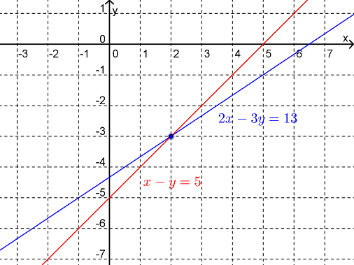
We can interpret the solution \((x,y)=(2,-3)\) as the point in the plane at which the straight lines represented by the equations \(2x-3y=13\) and \(x-y=5\) intersect.
Multiplying the second equation by \(2\) and then subtracting this from the first equation gives \(y=-3\text{.}\) Substituting this result into either of the original equations gives \(x=2\text{.}\) Thus the solution is \((x,y)=(2,-3)\text{.}\)
As shown in Figure 15.1.4, we can interpret the solution \((x,y)=(2,-3)\) as the point in the plane at which the straight lines represented by the equations \(2x-3y=13\) and \(x-y=5\) intersect. 
Example 15.1.5.
Solve the following system of linear equations and interpret the answer geometrically
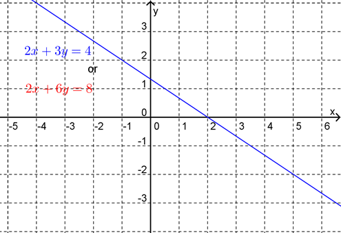
The solution set is \((x,y)=\left(t,\frac{4}{3}-\frac{2}{3}t\right)\text{.}\) The geometric interpretation of this system of linear equations is that both equations represent the same line.
Multiplying the first equation by \(2\) and then subtracting this from the second equation gives \(0=0\text{.}\) This tells us that any values of \(x\) and \(y\) that satisfy the first equation will also satisfy the second equation. Thus there are infinitely many solutions. We may choose \(x\) (say) to be anything we like, and then find a corresponding value for \(y\) (from either equation). So if we set \(x=t\text{,}\) then
and the solution set is
Thus, the parameter \(t\) labels the infinite family of solutions.
The geometric interpretation of this system of linear equations is that both equations represent the same line (as shown in Figure 15.1.6). 
we can see that the line passes through the point \(\left(0,\frac{4}{3}\right)\) and is parallel to the vector \(\left(1,-\frac{2}{3}\right)\text{.}\)
Example 15.1.7.
Solve the following system of linear equations and interpret the answer geometrically
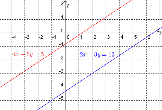
There are no solutions. Geometrically, this system of linear equations can be interpreted as two parallel lines in the plane.
Multiplying the first equation by \(2\) and then subtracting this from the second equation gives \(0=-21\text{.}\) This tells us that no values of \(x\) and \(y\) will satisfy these equations. Thus there are no solutions. A system of equations with no solution is said to be inconsistent.
Geometrically, this system of linear equations can be interpreted as two parallel lines in the plane, as shown in Figure 15.1.8. 
The above (simple) examples illustrate two important facts that hold for all systems of linear equations. Firstly:
Definition 15.1.9.
A system of \(m\) linear equations in \(n\) unknowns has either
A unique solution,
An infinite number of solutions, or
No solution
Thus it is impossible, for example, for a system of linear equations to have exactly two or exactly three solutions. (We will see why this is later.) Secondly, we cannot tell which of these cases (i.e. a unique solution, infinitely many solutions or no solution) applies simply by counting the number of equations and unknowns.
For systems of two linear equations in two unknowns we have seen that we can solve the system via the "substitution method" (viz. making one variable the subject of one equation and then substituting this into the second equation) or the "elimination method" (viz. adding a multiple of one equation to other). For larger system of equations this basic idea can still be used but the working can be become quite messy. In the following sections we will look at a systematic way of solving a system of \(m\) linear equations in \(n\) unknowns using matrices.