
Section 19.1 Introduction

Definition 19.1.1.

Let A be a square matrix of order \(n\text{.}\) The scalar \(\lambda\) is called an eigenvalue of \(A\) if there is a non-zero vector \(\mathbf{x}\) for which

\begin{equation*} A\mathbf{x}=\lambda \mathbf{x} \end{equation*}

\(\mathbf{x}\) is called an eigenvector of \(A\) associated with the eigenvalue \(\lambda\text{.}\)

For the matrix

\begin{equation*} A=\begin{pmatrix} 0 \amp 4 \amp 3 \\ \frac{1}{2} \amp 0 \amp 0 \\ 0 \amp \frac{1}{4} \amp 0 \end{pmatrix} \end{equation*}

determine if any of \(\mathbf{x}=\begin{pmatrix} 18 \amp 6 \amp 1 \end{pmatrix}^T \text{,}\) \(\mathbf{y}=\begin{pmatrix} -2 \amp 3 \amp 4 \end{pmatrix}^T \) or \(\mathbf{z}=\begin{pmatrix} 36 \amp 12 \amp 2 \end{pmatrix}^T \) are eigenvectors of \(A\text{.}\)

Answer.

\(\mathbf{x}\) and \(\mathbf{z}\) are eigenvectors of \(A\text{.}\)

Solution.

Since

\begin{equation*} A\mathbf{x}=\begin{pmatrix} 0 \amp 4 \amp 3 \\ \frac{1}{2} \amp 0 \amp 0 \\ 0 \amp \frac{1}{4} \amp 0 \end{pmatrix} \begin{pmatrix} 18 \\ 6 \\ 1 \end{pmatrix} = \begin{pmatrix} 27 \\ 9 \\ \frac{3}{2} \end{pmatrix} = \frac{3}{2}\begin{pmatrix} 18 \\ 6 \\ 1 \end{pmatrix} \end{equation*}

\(\mathbf{x}\) is an eigenvector of \(A\) associated with the eigenvalue \(\frac{3}{2}\text{.}\) Since

\begin{equation*} A\mathbf{y}=\begin{pmatrix} 0 \amp 4 \amp 3 \\ \frac{1}{2} \amp 0 \amp 0 \\ 0 \amp \frac{1}{4} \amp 0 \end{pmatrix} \begin{pmatrix} -2 \\ 3 \\ 4 \end{pmatrix} = \begin{pmatrix} 24 \\ -1 \\ \frac{3}{4} \end{pmatrix} \neq \lambda\begin{pmatrix} -2 \\ 3 \\ 4 \end{pmatrix} \end{equation*}

\(\mathbf{y}\) is not an eigenvector of \(A\text{.}\) Since

\begin{equation*} A\mathbf{z}=\begin{pmatrix} 0 \amp 4 \amp 3 \\ \frac{1}{2} \amp 0 \amp 0 \\ 0 \amp \frac{1}{4} \amp 0 \end{pmatrix} \begin{pmatrix} 36 \\ 12 \\ 2 \end{pmatrix} = \begin{pmatrix} 54 \\ 18 \\ 3 \end{pmatrix} = \frac{3}{2}\begin{pmatrix} 36 \\ 12 \\ 2 \end{pmatrix} \end{equation*}

\(\mathbf{z}\) is also an eigenvector of \(A\) associated with the eigenvalue \(\frac{3}{2}\text{.}\)

The matrix

\begin{equation*} A=\begin{pmatrix} 0 \amp 1 \\ 1 \amp 0 \end{pmatrix} \end{equation*}

is the matrix for the plane transformation of a reflection in the line \(y=x\text{.}\) Use this geometric interpretation of the matrix to determine the possible eigenvectors and eigenvalues of \(A\text{.}\)

Answer.

\(\mathbf{x}=t\begin{pmatrix} 1 \\ 1 \end{pmatrix}, \textrm{ where } t\in \mathbb{R}\) with eigenvalue \(1\text{.}\)

\(\mathbf{x}=t\begin{pmatrix} 1 \\ -1 \end{pmatrix}, \textrm{ where } t\in \mathbb{R}\) with eigenvalue \(-1\text{.}\)

Solution.

By definition eigenvectors satisfy the equation

\begin{equation*} A\mathbf{x}=\lambda\mathbf{x} \end{equation*}

Thinking in terms of transformations this equation says that an eigenvector will be a vector that is mapped by the transformation to some scalar multiple of itself, (i.e. to a vector parallel to itself). As illustrated in FigureĀ 19.1.4 any vector lying on the line \(y=x\) will be mapped to itself by a reflection in that line, i.e. for such vectors

\begin{equation*} A\mathbf{x}=\mathbf{x} \end{equation*}

Thus vectors of the form

\begin{equation*} \mathbf{x}=\begin{pmatrix} t \\ t \end{pmatrix}=t\begin{pmatrix} 1 \\ 1 \end{pmatrix}, \textrm{ where } t\in \mathbb{R} \end{equation*}

will be eigenvectors of \(A\) with an eigenvalue of \(1\text{.}\) (Note that we could check this algebraically if so desired.)

As also illustrated in FigureĀ 19.1.4, any vector perpendicular to the line \(y=x\) will be mapped by a reflection in that line to a vector of the same length but in the opposite direction, i.e. for such vectors

\begin{equation*} A\mathbf{x}=-\mathbf{x} \end{equation*}

Thus vectors of the form

\begin{equation*} \mathbf{x}=\begin{pmatrix} t \\ -t \end{pmatrix}=t\begin{pmatrix} 1 \\ -1 \end{pmatrix}, \textrm{ where } t\in \mathbb{R} \end{equation*}

will be eigenvectors of \(A\) with an eigenvalue of \(-1\text{.}\)
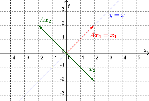
Figure 19.1.4.
Since no other vectors will be mapped by a reflection in the line \(y=x\) into scalar multiples of themselves, \(A\) will not have any more eigenvectors.

Given that \(\lambda=5\) is an eigenvalue for the matrix

\begin{equation*} A=\begin{pmatrix} 1 \amp 2 \\ 4 \amp 3 \end{pmatrix} \end{equation*}

find all eigenvectors associated with this eigenvalue.

Answer.

The eigenvectors associated with the eigenvalue \(\lambda=5\) are all scalar multiples of the vector \(\begin{pmatrix} 1 \amp 2 \end{pmatrix}^T\text{.}\)

Solution.

An eigenvector, \(\mathbf{x}\text{,}\) associated with the eigenvalue \(\lambda=5\) will satisfy the system of linear equations

\begin{equation*} A\mathbf{x}=5\mathbf{x} \end{equation*}

which can be rewritten as

\begin{align*} \begin{pmatrix} 1 \amp 2 \\ 4 \amp 3 \end{pmatrix} \begin{pmatrix} x_1 \\ x_2 \end{pmatrix} -5\begin{pmatrix} x_1 \\ x_2 \end{pmatrix} \amp =\begin{pmatrix} 0 \\ 0 \end{pmatrix}\\ \begin{pmatrix} x_1+2x_2-5x_1 \\ 4x_1+3x_2-5x_2 \end{pmatrix} \amp =\begin{pmatrix} 0 \\ 0 \end{pmatrix}\\ \begin{pmatrix} -4 \amp 2 \\ 4 \amp -2 \end{pmatrix} \begin{pmatrix} x_1 \\ x_2 \end{pmatrix} \amp =\begin{pmatrix} 0 \\ 0 \end{pmatrix} \end{align*}

Now, using Gauss Jordon elimination to solve this homogeneous system

\begin{equation*} \begin{pmatrix} -4 \amp 2 \amp 0 \\ 4 \amp -2 \amp 0 \end{pmatrix} \sim \begin{pmatrix} 2 \amp -1 \amp 0 \\ 0 \amp 0 \amp 0 \end{pmatrix} \begin{matrix} \hspace{5mm} R_1'=\frac{R_1}{-2} \\ \hspace{5mm} R_2'=R_2+R_1 \end{matrix} \end{equation*}

we see that this system has an infinite number of solutions which take the form

\begin{equation*} \mathbf{x}=\begin{pmatrix} x_1 \\ x_2 \end{pmatrix} \textrm{ where } 2x_1-x_2=0 \end{equation*}

or equivalently

\begin{equation*} \mathbf{x}=\begin{pmatrix} t \\ 2t \end{pmatrix}=t\begin{pmatrix} 1 \\ 2 \end{pmatrix} \end{equation*}

Thus the eigenvectors associated with the eigenvalue \(\lambda=5\) are all scalar multiples of the vector \(\begin{pmatrix} 1 \amp 2 \end{pmatrix}^T\text{.}\)

Of course, it is a good idea to check this result. Since

\begin{equation*} A\mathbf{x}=\begin{pmatrix} 1 \amp 2 \\ 4 \amp 3 \end{pmatrix} \begin{pmatrix} 1 \\ 2 \end{pmatrix}=\begin{pmatrix} 5 \\ 10 \end{pmatrix}=5\begin{pmatrix} 1 \\ 2 \end{pmatrix}=\lambda\mathbf{x} \end{equation*}

it is correct.