Section 1.1 Introduction
Have you ever wondered how your calculator actually calculates \(e^x\) or \(\sin(x)\) (or other non-polynomial functions) for particular values of \(x\text{?}\) Essentially, the way it is done is to write the function as an infinite series and then use as many terms of this series as necessary to obtain a value accurate to the number of digits in the calculator's display. For example, (as we will learn later on) the function \(e^x\) can be represented by the infinite series
Thus, to calculate \(e^{0.3}\) say, we could put \(x=0.3\) into the series. As the table below shows, as we use more and more terms from the series it seems that the sum isn't changing in the first few decimal places. Thus we might claim that to four decimal digits \(e^{0.3}=1.350\text{.}\)
| Number of Terms | Sum | Value |
|---|---|---|
| \(1\) | \(1\) | \(1\) |
| \(2\) | \(1+0.3\) | \(1.3\) |
| \(3\) | \(1+0.3+\dfrac{0.3^2}{2!}\) | \(1.345\) |
| \(4\) | \(1+0.3+\dfrac{0.3^2}{2!}+\dfrac{0.3^3}{3!}\) | \(1.3495\) |
| \(5\) | \(1+0.3+\dfrac{0.3^2}{2!}+\dfrac{0.3^3}{3!}+\dfrac{0.3^4}{4!}\) | \(1.3498375\) |
| \(6\) | \(1+0.3+\dfrac{0.3^2}{2!}+\dfrac{0.3^3}{3!}+\dfrac{0.3^4}{4!}+\dfrac{0.3^5}{5!}\) | \(1.3498775\) |
We call \(1, 1.3, 1.345, 1.3495, 1.3498375, 1.3498775, \ldots\) the sequence of partial sums for \(e^{0.3}\text{.}\)
Of course there are some really big questions here. Is it possible to find an infinite series representation for a given function? If so, how do we know that for any particular value of the independent variable the sum of more and more terms of the infinite series representation gets closer to the function value (or indeed any value at all)? These are the topics that we will address in this chapter.
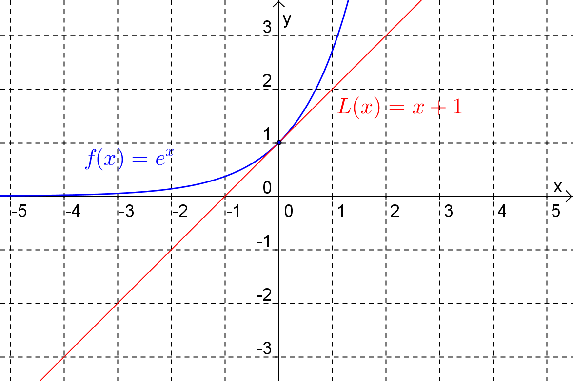
As a natural part of the discussion of the above questions we will also deal with the idea of approximating a function by a polynomial. We have seen previously (in Math1110) that near a given \(x\)-value a function can be approximated by its tangent. (We called such an approximation the linear approximation). For example, for values of \(x\) near \(0\) the function \(e^x\) can be approximated by the function \(L(x)=x+1\) which, as shown in Figure 1.1.1, is the tangent to the function at \(x=0\text{.}\)
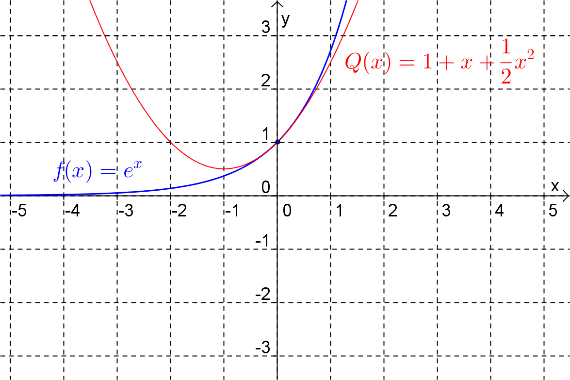
Notice that the linear approximation, \(L(x)\text{,}\) is the function obtained by truncating the infinite series representation for \(e^x\) (given above) after two terms. If we were to take the first three terms of the series we would have a quadratic approximation for \(e^x\text{,}\) i.e.
(See Figure 1.1.2.) By using more terms from the infinite expansion we can obtain higher order polynomial approximations which we hope will be more accurate over a greater interval around the point of tangency. The idea of approximating a function by a polynomial has many uses in mathematics besides that of being used in calculators.