Section 16.2 Interpretation Via Columns
Consider (initially at least) a system of two linear equations in two unknowns \(x\) and \(y\)
which can be represented by the augmented matrix
To give a geometric interpretation of this system of equations (in terms of the columns) we are going to think of the \(2\times 1\) matrix
as representing the vector in \(\mathbb{R}^2\) (i.e. in the plane) whose tail is at the origin and whose head is at the point \((v_1,v_2)\text{.}\) Thus this matrix is sometimes called a column vector.
Example 16.2.1.
The vector represented by \(\begin{pmatrix} 3 \\ 2 \end{pmatrix} \) is sketched in Figure 16.2.2. 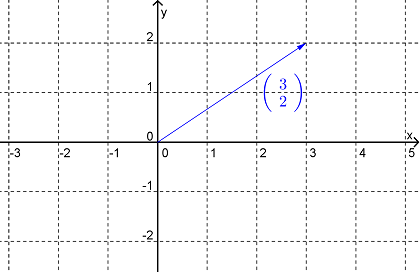
Now, the system of linear equations given above can be written as
or, if we let \(\mathbf{a_1} =\begin{pmatrix} a_{11} \\ a_{21} \end{pmatrix} \text{,}\) \(\mathbf{a_2}= \begin{pmatrix} a_{12} \\ a_{22} \end{pmatrix} \) and \(\mathbf{b} =\begin{pmatrix} b_{1} \\ b_{2} \end{pmatrix} \) as
Remember that when written in this form, the \(+\) sign means vector addition and \(x\mathbf{a_1}\text{,}\) for example, means the scalar multiplication of the vector \(\mathbf{a_1}\) by the scalar \(x\text{.}\) So solving this system of linear equations can be interpreted as finding scalars \(x\) and \(y\) such that the vector \(\mathbf{b}\) can be written in terms of the vectors \(\mathbf{a_1}\) and \(\mathbf{a_2}\text{.}\)
Example 16.2.3.
Solve the following system of linear equations and interpret your answer geometrically in terms of the columns of the augmented matrix.
The augmented matrix and its reduced row-echelon equivalent matrix are
Thus the solution is \((x,y)=\left(\frac{3}{2},2 \right)\text{.}\) Geometrically we can interpret this solution as saying the vector \(\begin{pmatrix} -3 \\ 7 \end{pmatrix}\) can be written in terms of the vectors \(\begin{pmatrix} 2 \\ 2 \end{pmatrix}\) and \(\begin{pmatrix} -3 \\ 2 \end{pmatrix}\) via the expression
See Figure 16.2.4. Note that the solution is also saying that there is only one way in which \(\begin{pmatrix} -3 \\ 7 \end{pmatrix}\) can be written in terms of \(\begin{pmatrix} 2 \\ 2 \end{pmatrix}\) and \(\begin{pmatrix} -3 \\ 2 \end{pmatrix}\text{.}\) 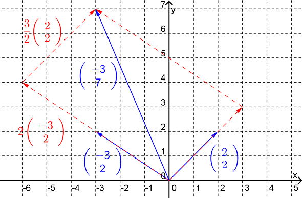
Before going on to consider systems of linear equations involving \(3\) (or more) variables it is convenient to introduce some new terminology.
Definition 16.2.5.
The vector \(a_1\mathbf{v_1}+a_2\mathbf{v_2}+\dots a_n\mathbf{v_n}\text{,}\) where \(a_i\in \mathbb{R}\text{,}\) is said to be a linear combination of the vectors \(\mathbf{v_1}, \mathbf{v_2}, \dots, \mathbf{v_n}\text{.}\)
The set of all linear combinations of the set of vectors \(\{\mathbf{v_1}, \mathbf{v_2}, \dots, \mathbf{v_n}\}\) is said to be the span of that set of vectors.
Example 16.2.6. (Example 16.2.3 cont.).
The geometric interpretation (in terms of the columns) of the system of linear equations
can be now be phrased as:
The vector \(\begin{pmatrix} -3 \\ 7 \end{pmatrix}\) can be written as a linear combination of the vectors \(\begin{pmatrix} 2 \\ 2 \end{pmatrix}\) and \(\begin{pmatrix} -3 \\ 2 \end{pmatrix}\text{,}\) and in only one way, or
The vector \(\begin{pmatrix} -3 \\ 7 \end{pmatrix}\) is in the span of the vectors \(\begin{pmatrix} 2 \\ 2 \end{pmatrix}\) and \(\begin{pmatrix} -3 \\ 2 \end{pmatrix}\text{.}\)
Example 16.2.7.
Describe the span of the set of vectors \(\left \{\mathbf{v_1, v_2} \right \}=\left \{\begin{pmatrix} 2 \\ 2 \end{pmatrix}, \begin{pmatrix} -3 \\ 2 \end{pmatrix} \right \}\text{.}\)
Solution.The span of the set \(\{\mathbf{v_1, v_2}\}\) is the set of vectors \(\mathbf{u}\) of the form
where \(x\) and \(y\) are scalars. From what we learnt about vectors in Math1110 we know that any vector in the plane will be able to be written as linear combination of these two vectors and hence the span of \(\{\mathbf{v_1, v_2}\}\) will be all vectors in \(\mathbb{R}^2\text{.}\) Alternatively, we could approach this problem algebraically. Let \(\mathbf{u}=\begin{pmatrix} a \\ b \end{pmatrix}\) be a vector in the span of \(\{\mathbf{v_1, v_2}\}\text{.}\) Then
Using Gauss Jordon elimination gives
and so the solution is \((x,y)=\left(\frac{a}{5}+\frac{3b}{10},\frac{b}{5}-\frac{a}{5}\right)\text{.}\) Thus, no matter which vector, \(\mathbf{u}\text{,}\) in \(\mathbb{R}^2\) we choose we can find the scalars so that \(\mathbf{u}\) is a linear combination of \(\mathbf{v_1}\) and \(\mathbf{v_2}\) and hence in the span of \(\{\mathbf{v_1, v_2}\}\text{.}\)
Example 16.2.8.
Describe the span of the set of vectors \(\{\mathbf{v_1, v_2}\}=\left \{\begin{pmatrix} 2 \\ 2 \\ 1 \end{pmatrix}, \begin{pmatrix} -3 \\ 2 \\ -1 \end{pmatrix} \right \}\text{.}\)
Solution.Firstly note that the vectors in this set are \(3\)-dimensional vectors and hence the vectors in the span will also be \(3\)-dimensional. Now, the span of the set \(\{\mathbf{v_1, v_2}\}\) is the set of vectors \(\mathbf{u}\) of the form
We recognise this as the vector equation of the plane through the origin and with direction vectors \(\mathbf{v_1}\) and \(\mathbf{v_2}\text{,}\) as shown in Figure 16.2.9. 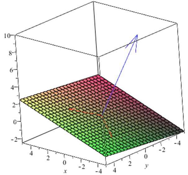
Thus the Cartesian equation of this plane is
Definition 16.2.10.
The set of vectors \(\mathbf{\{v_1, v_2, \dots, v_n\}}\) is called linearly independent if no vector in the set can be written as a linear combination of the other vectors in the set, or equivalently if the only solution to homogeneous system of linear equations
is \(a_1=a_2=\dots=a_n=0\text{.}\)
A set of vectors that is not linearly independent is called linearly dependent.
Example 16.2.11.
Decide if the following sets of vectors are linearly independent or not.
\(\displaystyle \{\mathbf{v_1, v_2, v_3}\}=\left \{\begin{pmatrix} 2 \\ 2 \end{pmatrix}, \begin{pmatrix} -3 \\ 2 \end{pmatrix}, \begin{pmatrix} -3 \\ 7 \end{pmatrix} \right \}\)
\(\displaystyle \{\mathbf{v_1, v_2}\}=\left \{\begin{pmatrix} 2 \\ 2 \end{pmatrix}, \begin{pmatrix} -3 \\ 2 \end{pmatrix} \right \}\)
This set of vectors is linearly dependent since (from our previous examples) we know that
\begin{equation*} \begin{pmatrix} -3 \\ 7 \end{pmatrix}=\frac{3}{2} \begin{pmatrix} 2 \\ 2 \end{pmatrix}+2\begin{pmatrix} -3 \\ 2 \end{pmatrix} \end{equation*}i.e. \(\mathbf{v_3}\) can be written as a linear combination of \(\mathbf{v_1}\) and \(\mathbf{v_2}\text{.}\)This set of vectors is linearly independent since the only solution to
\begin{equation*} x_1\mathbf{v_1}+x_2\mathbf{v_2}=\mathbf{0} \end{equation*}is \(x_1=x_2=0\text{.}\) Note that in this case this is telling us that \(\mathbf{v_2}\) is not a scalar multiple of \(\mathbf{v_1}\text{,}\) i.e. \(\mathbf{v_2}\) is not parallel to \(\mathbf{v_1}\text{.}\)
We are now ready to discuss the geometric interpretation, in terms of the columns, of a system of three linear equations in three unknowns \(x\text{,}\) \(y\) and \(z\text{,}\) i.e. of
This system of three linear equations can be written as
or, if we let \(\mathbf{a_1}= \begin{pmatrix} a_{11} \\ a_{21} \\ a_{31} \end{pmatrix}\text{,}\) \(\mathbf{a_2}= \begin{pmatrix} a_{12} \\ a_{22} \\ a_{32} \end{pmatrix}\text{,}\) \(\mathbf{a_3}= \begin{pmatrix} a_{13} \\ a_{23} \\ a_{33} \end{pmatrix}\) and \(\mathbf{b}= \begin{pmatrix} b_{1} \\ b_{2} \\ b_{3} \end{pmatrix}\) as
Thus, solving this system of linear equations can be interpreted as finding scalars \(x\text{,}\) \(y\) and \(z\) such that the vector \(\mathbf{b}\) can be written as a linear combination of the vectors \(\{\mathbf{a_1, a_2, a_3}\}\text{,}\) (or equivalently, that \(\mathbf{b}\) is in the span of \(\{\mathbf{a_1, a_2, a_3}\}\)).
Example 16.2.12.
Solve the following system of linear equations and interpret your answer geometrically in terms of the columns of the augmented matrix.
The augmented matrix and its reduced row-echelon equivalent matrix are
Thus the solution is \((x,y,z)=\left(\frac{3}{2},-1,2 \right)\text{.}\) The geometric interpretation of this solution is that the vector \(\begin{pmatrix} 3 \\ 6 \\ 3 \end{pmatrix}\) (shown in blue in Figure 16.2.13) can be written as a linear combination of the vectors \(\left \{\begin{pmatrix} 2 \\ 2 \\ 4 \end{pmatrix}, \begin{pmatrix} 4 \\ 3 \\ 1 \end{pmatrix}, \begin{pmatrix} 2 \\ 3 \\ -1 \end{pmatrix} \right \}\) (shown in red in Figure 16.2.13) and in only one way, (shown in green in Figure 16.2.13). 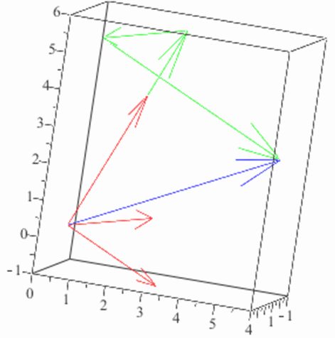
Note that if the system of linear equations is homogeneous (i.e. \(\mathbf{b=0}\)) then the solution of the system tells us if the set of vectors \(\{\mathbf{a_1, a_2, a_3}\}\) is linearly independent or not.
Example 16.2.14.
Solve the following system of linear equations and interpret your answer geometrically in terms of the columns of the augmented matrix.
The augmented matrix and its reduced row-echelon equivalent matrix are
Thus the solution is \((x,y,z)=(0,0,0)\text{.}\) The geometric interpretatifon of this solution is that the column vectors of the coefficient matrix are linearly independent, i.e. that no one of those vectors can be written in terms of the other two. If the column vectors had turned out to be linearly dependent then we could have written, for example,
This would imply that \(\mathbf{a_3}\) lies in the plane defined by the vectors \(\mathbf{a_1}\) and \(\mathbf{a_2}\text{,}\) or to say the same thing, that \(\mathbf{a_1}\text{,}\) \(\mathbf{a_2}\) and \(\mathbf{a_3}\) are coplanar. Since the vectors are linearly independent we can say these vectors are not coplanar. See Figure 16.2.15. 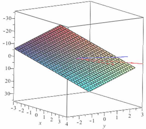
Example 16.2.16.
Solve the following system of linear equations and interpret your answer geometrically in terms of the columns of the augmented matrix.
The augmented matrix and its reduced row-echelon equivalent matrix are
Thus this system has an infinite number of solutions given by
To discuss the geometric interpretation of this solution let
Then we can say that \(\mathbf{b}\) can be written as a linear combination of the vectors \(\{\mathbf{a_1, a_2, a_3}\}\) in an infinite number of ways. Notice that with \(t=0\) we have
Since \(\mathbf{b}\) can written as a linear combination of \(\{\mathbf{a_1, a_2}\}\text{,}\) the vectors \(\mathbf{b}\text{,}\) \(\mathbf{a_1}\) and \(\mathbf{a_2}\) are coplanar. Similarly (with \(t=-2\)) we can see that \(\mathbf{b}\text{,}\) \(\mathbf{a_1}\) and \(\mathbf{a_3}\) are coplanar. So, in fact, \(\mathbf{b}\text{,}\) \(\mathbf{a_1}\text{,}\) \(\mathbf{a_2}\) and \(\mathbf{a_3}\) are all coplanar.
Finally we can see from the above working that the vectors \(\{\mathbf{a_1, a_2, a_3}\}\) are linearly dependent since if \(\mathbf{b=0}\) then the reduced row-echelon form would be
To summarise what we have we have covered:
Definition 16.2.17.
Consider the system of linear equations whose augmented matrix is
The following statements are equivalent:
The system has a unique solution
The planes represented by the rows intersect in a point
The column vectors of the coefficient matrix are linearly independent
Exercises Example Tasks
1.
Decide if the following sets of vectors are linearly independent or not
\(\displaystyle \{\mathbf{v_1, v_2}\}=\left \{(1,1), (1,-1)\right \}\)
\(\displaystyle \{\mathbf{v_1, v_2, v_3}\}=\left \{(1,1, 2), (1,-1,0), (3,2,1)\right \}\)
2.
Solve the following system of linear equations and interpret your answer geometrically in terms of the columns of the augmented matrix.
3.
Show that the set of vectors \(\left \{(2,3, 7), (3,4, 5), (2,1,-15) \right\}\) are linearly dependent.
Find values of \(a\text{,}\) \(b\) and \(c\) such that the following system of linear equations has infinitely many solutions
\begin{align*} 2x_1+3x_2+2x_3 \amp =a\\ 3x_1+4x_2+x_3 \amp =b\\ 7x_1+5x_2-15x_3 \amp =c \end{align*}