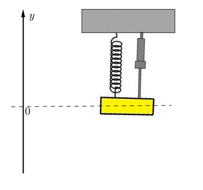
Imagine now that some sort of damping mechanism is added to the object-spring system as shown in Figure 14.2.1. (Such a system might be used as a simple model of a car shock absorber for example.)
Figure14.2.1. So long as the speed of the object is not too fast then a reasonable assumption is that the damping force acting on the object, \(\mathbf{F_d}\text{,}\) is proportional to the speed and acts in the direction opposing the motion of the object. Thus
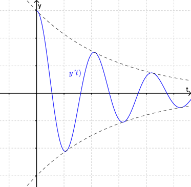
Thus the nature of the general solution to (14.2.1) depends upon the sign of \(p^2-q^2\text{,}\) or equivalently, on the magnitude of the parameter \(\delta=\frac{p}{q}\text{.}\)\(\delta\) is called the damping parameter of the system.
If \(p^2-q^2\gt 0\) (or equivalently \(\delta=\frac{p}{q}\lt 1\)) then the general solution is
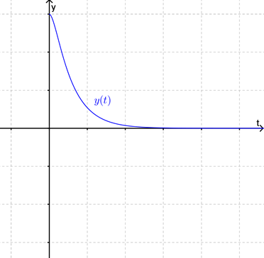
where both \(r_1\) and \(r_2\) are negative and hence the function will be like that shown in Figure 14.2.3. In this case the system is called over-damped.
Figure14.2.3. Finally if \(p^2-q^2=0\) (or equivalently \(\delta=\frac{p}{q}=1\)) then the general solution is
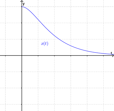
and hence the function will be like that shown in Figure 14.2.4. In this case the system is called critically-damped.
Figure14.2.4. The critically-damped case is of practical interest. Often we want to add damping to a system so that it returns close to its equilibrium position "as quickly as possible", (for example in the shock absorber of a car). It turns out that this is achieved by critical damping.