Section 7.1 Critical Points
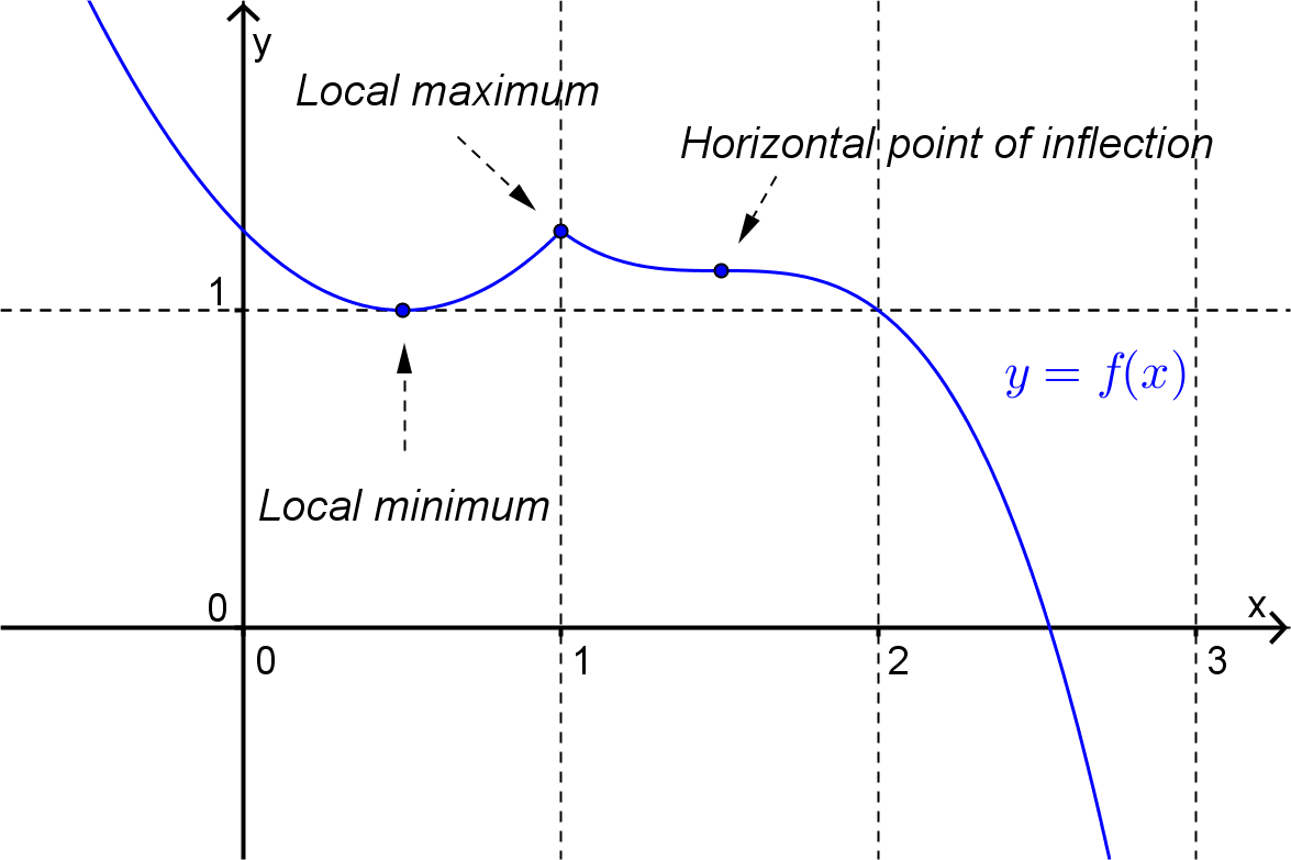
Recall that a function of one variable, \(f(x)\) has a “critical point” at \(x=x_0\) if the tangent line to the curve at \(x=x_0\) is horizontal or if the derivative does not exist at that point. This critical point can be either a (local) maximum, minimum or horizontal point of inflection or vertical point of inflection. (The first three possibilities are shown in Figure 7.1.1 below.)
The idea of critical points can be applied to functions of two variables.
Definition 7.1.2. Critical Point.
The function \(z=f(x,y)\) has a critical point at \((x_0,y_0)\) if the tangent plane to the surface at the point \((x_0,y_0,z_0)\) is horizontal or if one of the directional derivatives does not exist.
As with functions of one variable, critical points of functions of two variables will be one of three types.
If at a critical point \(f(x,y) \leq f(x_0,y_0)\) for all points in some open disk centred on \((x_0,y_0)\) then the critical point is a local maximum.
If at a critical point \(f(x,y) \geq f(x_0,y_0)\) for all points in some open disk centred on \((x_0,y_0)\) then the critical point is a local minimum.
For a smooth function (i.e. a function for which all derivatives exist) if a critical point is not a local maximum or a local minimum then it is a saddle point.
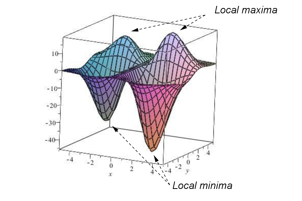
Example 7.1.3.
The graph of the function
is given below with local maxima and local minima labelled.
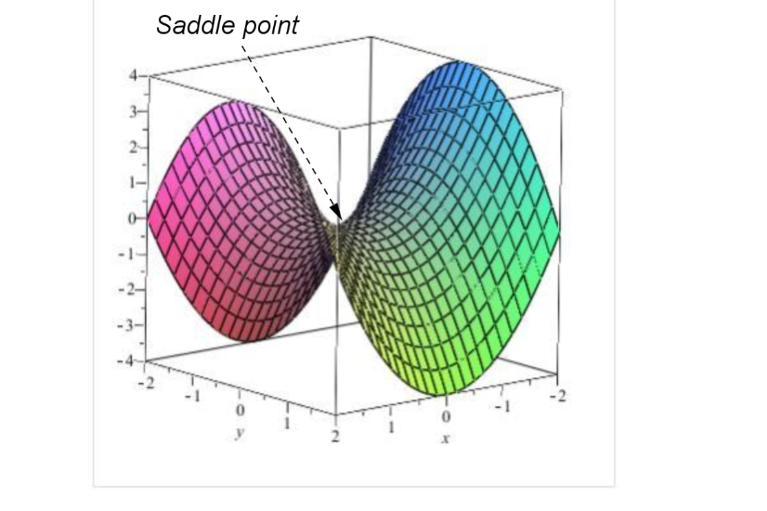
Example 7.1.5.
The graph of the function \(f(x,y) = x^2-y^2\) is given below with a saddle point labelled.
For smooth functions we can find the critical points by looking for those points where the tangent plane is horizontal. If the function \(z=f(x,y)\) has a tangent plane at the point \((x_0,y_0,z_0)\) we can determine algebraically that it is horizontal by checking that:
The normal vector for the plane is parallel to the vector \(\langle 0,0,1 \rangle\text{,}\) or
The directional derivative at \((x_0,y_0)\) is zero in every direction, or
The gradient vector at \((x_0,y_0)\) is \(\langle 0,0 \rangle\text{.}\)
These conditions are all equivalent and they lead us to the following theorem.
Theorem 7.1.7. Critical Point.
The point \((x_0,y_0)\) is a critical point of the function \(z = f(x,y)\) if
or, if at least one of these derivatives does not exist.
Note: For the most part, we will assume that the function is smooth, i.e. has derivatives of all orders. In particular a smooth function does not have any discontinuities or cusps. Such critical points will occur for functions of two variables when at least one of the partial derivatives does not exist at the critical point.
Example 7.1.8.
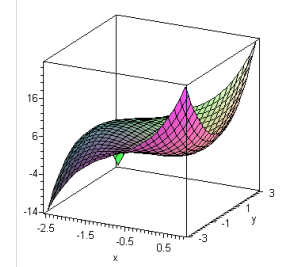
Locate, and determine the nature of, the critical points of the function
\(\left(0,0\right)\) is a local minimum; \(\left(-\dfrac{5}{3},0\right)\) is a local maximum; \(\left(-1,2\right)\) and \(\left(-1,-2\right)\) are saddle points.
To locate the critical points we solve the equations \(z_x = z_y = 0\text{,}\) and check for any points where they do not exist. Since this function is given by a polynomial, the partial derivatives exist. We set them to zero below.
From (7.1.2)
Putting \(y=0\) into (7.1.1) gives
Putting \(x=-1\) into (7.1.1) gives
Thus there are 4 critical points at
If we have the graph of the function then we can usually determine the nature of these critical points by inspection. From the (computer generated) graph shown below we can see with very careful inspection that the critical point at \((0,0)\) is a local minimum, the critical point at \(\left( -\dfrac{5}{3}, 0 \right)\) is a local maximum and the critical points at \((-1,2)\) and \((-1,-2)\) are saddle points.
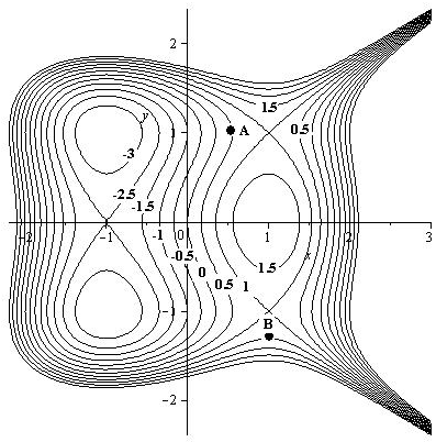
Sometimes the nature of the critical points is not clear on such graphs or we don't have access to the graph. Another approach to determining the nature of the critical points is to sketch the level curves for the function.
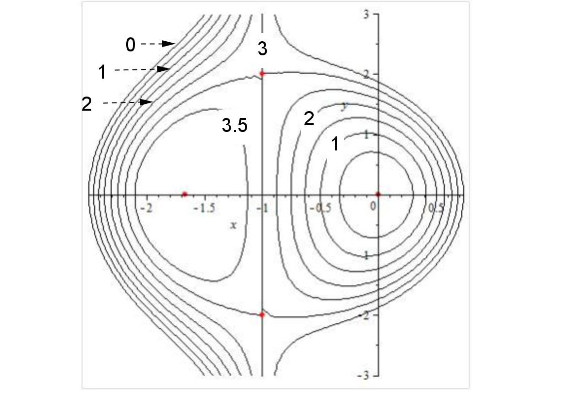
From this diagram we can see that as we move away from the critical points at \(\left(0,0\right)\) in any direction the function value is increasing and hence \(\left(0,0\right)\) is local minimum. Similarly as we move away from the critical point at \(\left(-\dfrac{5}{3},0\right)\) in any direction the function value is decreasing is hence \(\left(-\dfrac{5}{3},0\right)\) is a local maximum. For the critical points at \(\left(-1,2\right)\) and \(\left(-1,-2\right)\) we can move away in some directions and have the function value increase while in other directions the function value will decrease. Hence these critical points are saddle points.
Exercises Example Tasks
1.
Find the critical points of the function \(f(x,y) = 3x-x^3-2y^2+y^4\) and use the plot of level curves given below to determine the nature of each critical point.