Section 20.2 Coupled Linear Differential Equations
Recall that the linear differential equation
has the solution (via separation of variables)
where \(C\) is an arbitrary constant. Consider now the system of two linear differential equations
where \(a, \, b, \, c, \, d \in \mathbb{R}\text{,}\) which can be written in matrix notation as
where \(\mathbf{x} = \begin{pmatrix} x_1 \\ x_2 \end{pmatrix}\text{,}\) \(\dot{\mathbf{x}} = \begin{pmatrix} \dot{x}_1 \\ \dot{x}_2 \end{pmatrix}\) and \(A = \begin{pmatrix} a \amp b \\ c \amp d \end{pmatrix}\text{.}\) These equations are “coupled”, i.e. the derivative of \(x_1(t)\) depends on both \(x_1(t)\) and \(x_2(t)\) and likewise for the derivative of \(x_2(t)\text{.}\) Thus we can't solve the first equation unless we can solve the second and vice versa. Note that if \(A\) is diagonal then the equations become uncoupled and we could solve each separately.
If the matrix \(A\) has 2 distinct eigenvalues, \(\lambda_1\) and \(\lambda_2\text{,}\) by making the change of variable \(\mathbf{y}= P^{-1} \mathbf{x}\text{,}\) where \(P\) is the matrix whose columns are the eigenvectors \(\mathbf{v_1}\) and \(\mathbf{v_2}\) of \(A\text{,}\) we can transform (20.2.1) into a system where the matrix is diagonal. By solving that system and converting back to our original variables we find that the general solution to (20.2.1) is
where \(C_1\) and \(C_2\) are arbitrary constants. We can check that (20.2.2) is indeed a solution to (20.2.1). From (20.2.2)
and
Example 20.2.1.
Find the solution to the initial value problem
where \(x_1(0) = 2\) and \(x_2(0) = 3\text{.}\)
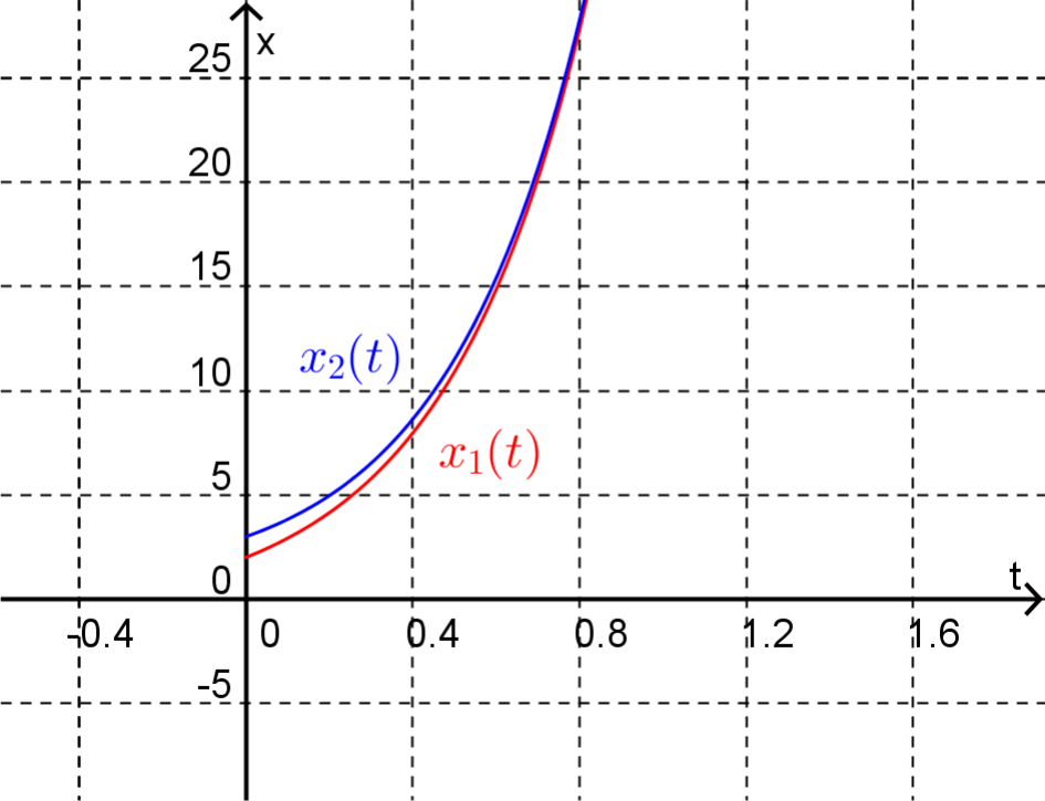
\(x_1(t) = \dfrac{5}{2} e^{3t} - \dfrac{1}{2} e^{-t}\) and \(x_2(t) = \dfrac{5}{2} e^{3t} + \dfrac{1}{2} e^{-t}\)
In matrix notation this system is
The eigenvalues of \(\begin{pmatrix} 1 \amp 2 \\ 2 \amp 1 \end{pmatrix}\) turn out to be \(\lambda_1 = -1\) and \(\lambda_2 = 3\) with associated eigenvectors \(\mathbf{v_1} = \begin{pmatrix} 1 \\ -1 \end{pmatrix}\) and \(\mathbf{v_2} = \begin{pmatrix} 1 \\ 1 \end{pmatrix}\text{.}\) Thus, from (20.2.2) the general solution is
From the initial conditions we have
Solving this system of linear equations (by Gauss-Jordan elimination say) gives
Thus, the solution to the initial value problem is
or equivalently
Note that you can always check your answer by checking that the functions do indeed satisfy the original equations.
Figure 20.2.2 shows the graph of these solutions. Notice that as \(t\) gets larger because of the \(e^{-t}\) term in each solution the functions get closer together and because of the \(e^{3t}\) term both solutions grow (exponentially). Thus the eigenvalues of the matrix \(A\) will give us some idea of the qualitative nature of the solutions.
Example 20.2.3.
Solve the initial value problem
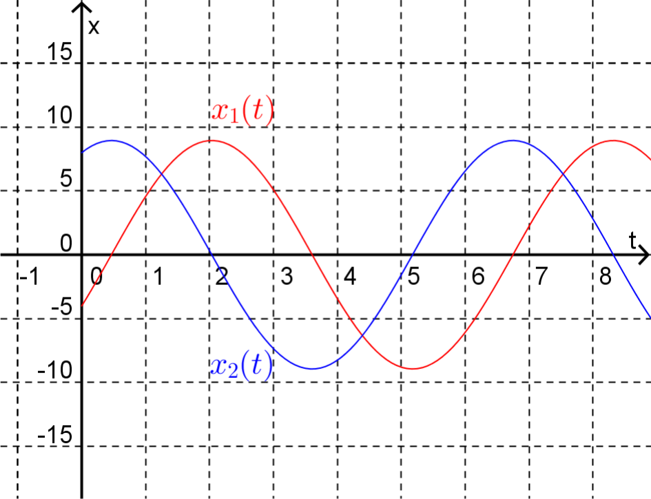
\(\mathbf{x} = \begin{pmatrix} 8 \sin(t) - 4 \cos(t) \\ 8 \cos(t) + 4 \sin(t) \end{pmatrix}\)
The eigenvalues of \(A\) turn out to be purely complex with \(\lambda_1 = i\) and \(\lambda_2 = -i\text{.}\) The associated eigenvectors are \(\mathbf{v_1} = \begin{pmatrix} -i \\ 1 \end{pmatrix}\) and \(\mathbf{v_2}= \begin{pmatrix} i \\ 1 \end{pmatrix}\text{.}\) Thus, from (20.2.2) the general solution is
From the initial conditions we have
which upon solving gives
Thus, the solution to the initial value problem is
We can simplify this solution by using Euler's equation
Thus
which simplifies to
This is a real solution! As explained below, because all of the entries in \(A\) are real and the initial conditions are real the solution will also be real.
As shown in Figure 20.2.4 where these solutions are graphed, purely complex eigenvalues are associated with periodic solutions. The period of these solutions is \(\dfrac{2 \pi}{| \operatorname{Im}(\lambda) |}\text{.}\)
Consider the system of coupled linear differential equations
where the entries in \(A\) are all real. Now imagine that this system has a complex solution given by
Taking the complex conjugates of both sides of (20.2.3)
Since \(\bar{\dot{\mathbf{x}}} = \dot{\bar{\mathbf{x}}}\) and \(\bar{A} = A\) (as the entries in \(A\) are all real),
i.e.
will also be a solution to (20.2.3). Substituting (20.2.4) into (20.2.3) gives
while substituting (20.2.5) into (20.2.3) gives
Now, adding equations (20.2.6) and (20.2.7) gives
while subtracting (20.2.7) from (20.2.6) gives
Thus if we have a complex solution to (20.2.3) then both the real and imaginary parts of this complex solution must separately be solutions and hence a general solution to (20.2.3) is
This gives us another way of proceeding when the eigenvalues of \(A\) are complex.
Example 20.2.5.
Find the general solution to
\(\mathbf{x} = C_1 e^{2t} \begin{pmatrix} -5\cos(3t) \\ \cos(3t) - 3 \sin(3t) \end{pmatrix} + C_2 e^{2t} \begin{pmatrix} -5\sin(3t) \\ \sin(3t) + 3\cos(3t) \end{pmatrix}\)
Here the eigenvalues of \(A\) are complex with \(\lambda_1 = 2+3i\) and \(\lambda_2 = 2-3i\text{.}\) The eigenvector associated with \(\lambda_1\) is \(\mathbf{v_1} = \begin{pmatrix} -5 \\ 1+3i \end{pmatrix}\text{.}\) Thus, one solution to the system is
Simplifying this solution using Euler's equation gives
Since we know that both the real part and the imaginary part are solutions to the system we know that the general solution is
Figure 20.2.6 shows a plot of this solution when \(C_1 = C_2 = 1\text{.}\)
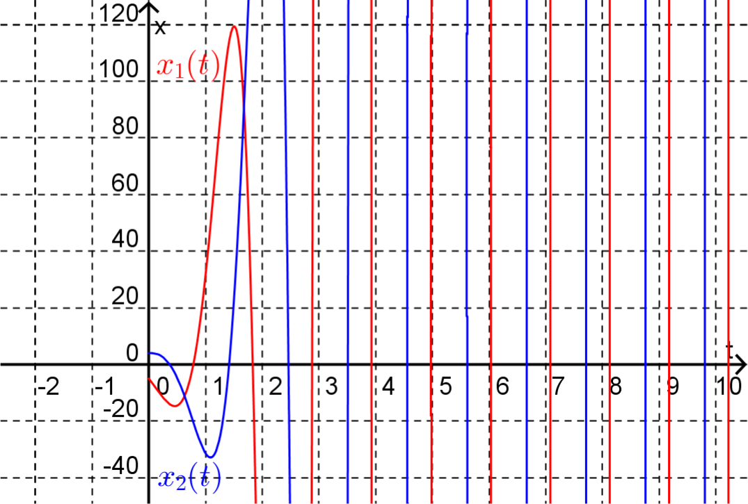
Note the solutions to the system are periodic with the period determined from the imaginary part of the eigenvalue. However, since the real part of the eigenvalue is positive the amplitude of the solutions grows without bound.
The discussion so far has concentrated on systems of two coupled first-order linear differential equations. However the ideas carry over to systems with more equations.
Theorem 20.2.7.
Consider the system of n coupled first-order linear differential equationsA qualitative description of the solutions to the system can be determined from the eigenvalues of \(A\text{.}\)
Remark 20.2.8.
If \(A\) has a positive real eigenvalue then the corresponding solution grows without bound.
If \(A\) has a negative real eigenvalue then the corresponding solution decays.
If \(A\) has a zero eigenvalue then the corresponding solution is constant.
If \(A\) has a pair of complex conjugate eigenvalues then the corresponding solution oscillates with period \(2\pi / \operatorname{Im}(\lambda)\) and with the amplitude either growing \((\operatorname{Re}(\lambda) > 0)\text{,}\) decaying \((\operatorname{Re}(\lambda) < 0 )\) or staying the same \((\operatorname{Re}(\lambda) = 0)\text{.}\)
Exercises Example Tasks
1.
Describe the long term behaviour of the solutions to the system \(\dot{\mathbf{x}} = A \bm{x}\text{,}\) where