Direction Fields and Euler's Method

Section 9.2 Direction Fields and Euler's Method

So far, the only methods that we have seen for actually solving a DE are anti-differentiation and guess and check. Clearly, these methods are very limited in their scope. Before looking at some methods for finding solutions to DEs in closed form, we will look at two methods by which we can approximate solutions to first order DEs, i.e. to DEs of the form

\begin{equation*} y'=f(x,y) \end{equation*}

Section 9.2.1 Direction Fields

The first method that we will look at aims to "draw" the solutions to the DE. If \(y(x)\) is the solution to the DE that passes through the point \((x_0,y_0)\) then the slope of the tangent to \(y(x)\) at \((x_0,y_0)\) is \(f(x_0,y_0)\text{.}\) So if we draw a small line segment passing through the point \((x_0,y_0)\) with slope \(f(x_0,y_0)\) (i.e. a small part of the tangent line) this will approximate the graph of the solution at this point. A plot showing these small line segments for many points is called a direction field for the DE.

Example 9.2.1.

Sketch the direction field for the DE

\begin{equation*} 3y'+y=x \end{equation*}

Use this direction field to sketch the graph of the solution to the DE satisfying the initial condition \(y(0)=2\text{.}\)

Solution.

Rearranging this first order DE in the form \(y'=f(x,y)\) gives

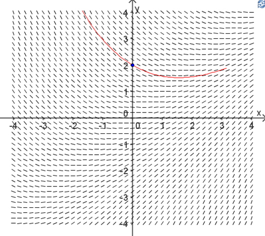
\begin{equation*} y'=\frac{x-y}{3}\text{,} \end{equation*}

i.e. \(f(x,y)=\frac{x-y}{3}\text{.}\) Now, at the point \((0,2)\) the slope of the tangent to \(y(x)\) will be

\begin{equation*} f(0,2)=\frac{0-2}{3}=-\frac{2}{3} \end{equation*}

So draw a small segment of the line passing through the point \((0,2)\) with slope \(-\frac{2}{3}\text{,}\) as shown in Figure 9.2.2.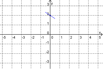

Repeating for many points \((x,y)\) in the plane gives the direction field for the DE shown in Figure 9.2.3.

Notice that from this direction field we can see the general shape of the family of solutions to the DE. We can also sketch any particular solution that we want. The particular solution satisfying \(y(0)=2\) has been constructed in Figure 9.2.3.

Example 9.2.4.

Sketch the direction field for the DE

\begin{equation*} \frac{dy}{dt}=y(1-y) \end{equation*}

Describe the long term behaviour of the solutions to this DE.

Note: A first order DE is called autonomous if it is of the form

\begin{equation*} \frac{dy}{dt}=f(y) \end{equation*}

and so this is an example of a first order autonomous DE.

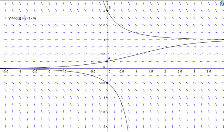
Solution.

Notice that for this DE the functions

\begin{equation*} y(x)=0 \textrm{ and } y(x)=1 \end{equation*}

are solutions and that for these solutions \(y'=0\text{.}\) (These solutions are called steady state solutions since \(y\) does not vary along these solutions). Notice also that at any point whose \(y\) coordinate is greater than \(1\text{,}\) \(y'\lt 0\text{.}\) Similarly for those points with \(y\) coordinate satisfying \(0\lt y\lt 1\text{,}\) \(y'>0\) and for those points with \(y\) coordinate satisfying \(y\lt 0\text{,}\) \(y'\lt 0\text{.}\) These observations allow us to very quickly make a sketch of the direction field. The direction field for this DE is shown in Figure 9.2.5.

From the direction field we can see that the behaviour of the solution for large values of \(x\) depends on the initial condition that the solution satisfies. If \(y(0)\lt 0\) then \(y\rightarrow -\infty\) as \(x\rightarrow\infty\) whereas if \(y(0)>0\) then \(y\rightarrow 1\) as \(x\rightarrow\infty\text{.}\)

Section 9.2.2 Euler's Method

The second method that we will look at aims to approximate the solution to the initial-value problem

\begin{equation*} y'=f(x,y), \hspace{5mm} y(x_0)=y_0 \end{equation*}

numerically (i.e to produce a table of values for the function). Given a point \((x_n,y_n)\) on the graph of the solution \(y(x)\text{,}\) Euler’s method approximates the next point \((x_{n+1},y_{n+1})\) on the graph of \(y(x)\) using the linear approximation

\begin{equation*} \Delta y=f(x_n,y_n)\Delta x \end{equation*}

Thus if \(x_{n+1}=x_n+\Delta x\text{,}\) where \(\Delta x\) is small, then

\begin{equation*} y_{n+1}=y_n+f(x_n,y_n)\Delta x \end{equation*}

Definition 9.2.1. Euler's Method (for solving the initial-value problem \(y'=f(x,y), \hspace{5mm} y(x_0)=y_0\)).

Choose a step size \(\Delta x\)
Begin at the point \((x_0,y_0)\)
Move from one point \((x_0,y_0)\) on the solution to the next point \((x_{n+1},y_{n+1})\) on the solution by:
\begin{align*} x_{n+1} \amp =x_n+\Delta x\\ y_{n+1} \amp =y_n+f(x_n,y_n)\Delta x \end{align*}

Note that the accuracy of Euler's method will depend on both the step size used and the distance from the initial known point on the solution.

Example 9.2.2.

Consider the initial-value problem:

\begin{equation*} y'=y, \hspace{5mm} y(0)=1 \end{equation*}

Estimate \(y(1)\) using Euler's method with step size

\(\displaystyle \Delta x=1\)
\(\displaystyle \Delta x=0.5\)
\(\displaystyle \Delta x=0.25\)

Answer.

\(y(1)=2\text{.}\)
\(y(1)=2.25\text{.}\)
\(\displaystyle y(1)=2.4414 \textrm{ (to 4 d.p.)}\)

Solution.

Here \(f(x,y)=y\text{.}\)

Let \((x_0,y_0)=(0,1)\text{.}\) Then with \(\Delta x=1\) we have
\begin{align*} x_1 \amp =x_0+\Delta x=0+1=1\\ y_1 \amp =y_0+f(x_0,y_0)\Delta x\\ \amp = 1+f(0,1)\times 1\\ \amp = 1+1\\ \amp = 2 \end{align*}
Thus the Euler estimate is \(y(1)=2\text{.}\)
Again, begin with \((x_0,y_0)=(0,1)\text{.}\) Using \(\Delta x=0.5\) we will need two iterations to reach \(x=1\text{.}\) The first iteration gives
\begin{align*} x_1 \amp =x_0+\Delta x=0+0.5=0.5\\ y_1 \amp =y_0+f(x_0,y_0)\Delta x\\ \amp = 1+f(0,1)\times 0.5\\ \amp = 1.5 \end{align*}
Now complete the second iteration
\begin{align*} x_2 \amp =x_1+\Delta x=0.5+0.5=1\\ y_2 \amp =y_1+f(x_1,y_1)\Delta x\\ \amp = 1.5+f(0.5,1.5)\times 0.5\\ \amp = 1.5+1.5\times 0.5\\ \amp = 2.25 \end{align*}
Thus the Euler estimate is \(y(1)=2.25\text{.}\)

With \(\Delta x=0.25\) we will need 4 iterations to reach \(x=1\text{.}\) We can conveniently summarise the calculations via a table

Table 9.2.3.

\(n\)	\(x_n\)	\(y_n\)	\(f(x_n,y_n)\)	\(f(x_n,y_n)\Delta x\)
\(0\)	\(0\)	\(1\)	\(1\)	\(0.25\)
\(1\)	\(0.25\)	\(1.25\)	\(1.25\)	\(0.3125\)
\(2\)	\(0.5\)	\(1.5625\)	\(1.5625\)	\(0.390625\)
\(3\)	\(0.75\)	\(1.953125\)	\(1.953125\)	\(0.48828125\)
\(4\)	\(1\)	\(2.44140625\)	\(\)

Thus the Euler estimate is \(y(1)=2.4414 \textrm{ (to 4 d.p.)}\)

Note that the exact solution to this initial-value problem is \(y=e^x\) and hence \(y(1)=e=2.7183\) (to 4 d.p.). Figure 9.2.4 shows how the Euler solution with \(\Delta x=0.5\) compares with the exact solution.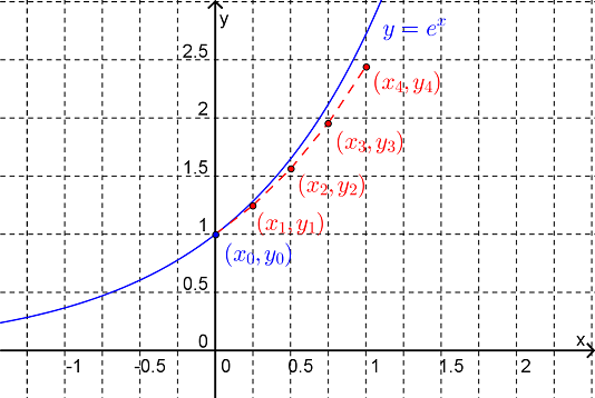

Example 9.2.5.

Consider the DE

\begin{equation*} y'=y+x^2, \hspace{5mm} y(1)=2 \end{equation*}

Use Euler's method with \(\Delta x=0.5\) to estimate \(y(3)\text{.}\)

Answer.

\(y(3)=20.4688 \textrm{ (to 4 d.p.)}\)

Solution.

Using the table layout:

Table 9.2.6.

\(n\)	\(x_n\)	\(y_n\)	\(f(x_n,y_n)\)	\(f(x_n,y_n)\Delta x\)
\(0\)	\(1\)	\(2\)	\(3\)	\(1.5\)
\(1\)	\(1.5\)	\(3.5\)	\(5.75\)	\(2.875\)
\(2\)	\(2\)	\(6.375\)	\(10.375\)	\(5.1875\)
\(3\)	\(2.5\)	\(11.5625\)	\(17.8125\)	\(8.9063\)
\(4\)	\(3\)	\(20.4688\)

Thus the Euler estimate is \(y(3)=20.4688 \textrm{ (to 4 d.p.)}\)

Exercises Example Tasks

1.

At time \(t\) the population density of the Striped Dingbat is modelled by the function \(P(t)\text{.}\) This function satisﬁes the DE

\begin{equation*} \frac{dP}{dt}=kP(C-P) \end{equation*}

where \(k\) and \(C\) are positive constants.

Find all steady-state solutions to this DE.
By considering the direction ﬁeld, explain how this model predicts the long-term Striped Dingbat population.

2.

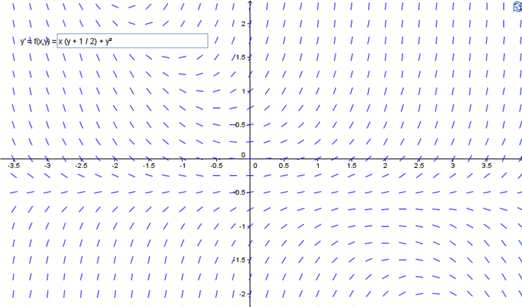
The direction field for the DE

\begin{equation*} y'=x\left(y+\frac{1}{2}\right)+y^2 \end{equation*}

is shown below. Sketch the solution satisfying the initial condition

\(\displaystyle y(0)=0.5\)
\(\displaystyle y(0)=-0.5\)

3.

Consider the initial-value problem

\begin{equation*} y'=xy+x, \hspace{5mm} y(0)=1 \end{equation*}

Use Euler's method with \(\Delta x=0.1\) to estimate \(y(0.3)\text{.}\)